This article delves into the intricate details of the AlphaFold algorithm, exploring its components, data sources, training regimen, and inference process. It also touches on related legal aspects and references to computational tools such as Kohl’s implementation of the algorithm. This guide aims to provide a comprehensive understanding for those new to the field of protein structure prediction.
Inside the AlphaFold Algorithm
AlphaFold’s algorithm is a complex interplay of several key components, each contributing to the accurate prediction of protein structures. Detailed explanations of these components can be found in the original publication’s Supplementary Methods 1.1–1.10. Pseudocode is available in Supplementary Information Algorithms 1–32, network diagrams in Supplementary Figs. 1–8, input features in Supplementary Table 1, and additional details in Supplementary Tables 2 and 3. Training and inference details are provided in Supplementary Methods 1.11–1.12 and Supplementary Tables 4 and 5.
The Invariant Point Attention (IPA) Module
The IPA module is a core component, merging pair representation, single representation, and geometric representation to refine the single representation. This module operates in 3D space, where each residue generates query, key, and value points within its local frame. These points are then projected into a global frame, allowing them to interact with each other. Finally, the resulting points are projected back into the local frame. This intricate process ensures invariance to the global frame. The affinity computation in 3D space relies on squared distances, and the coordinate transformations maintain the module’s invariance. For a deep dive into the algorithm, the proof of invariance, and a description of the multi-head version, refer to Supplementary Methods 1.8.2, titled ‘Invariant point attention (IPA)’. A similar approach, utilizing classic geometric invariants for pairwise feature construction instead of learned 3D points, has been applied to protein design.
Standard dot product attention is also computed on the abstract single representation, along with specialized attention on the pair representation. The pair representation enhances both the logits and values of the attention process, acting as the primary control mechanism for structure generation.
Data Sources and Inputs
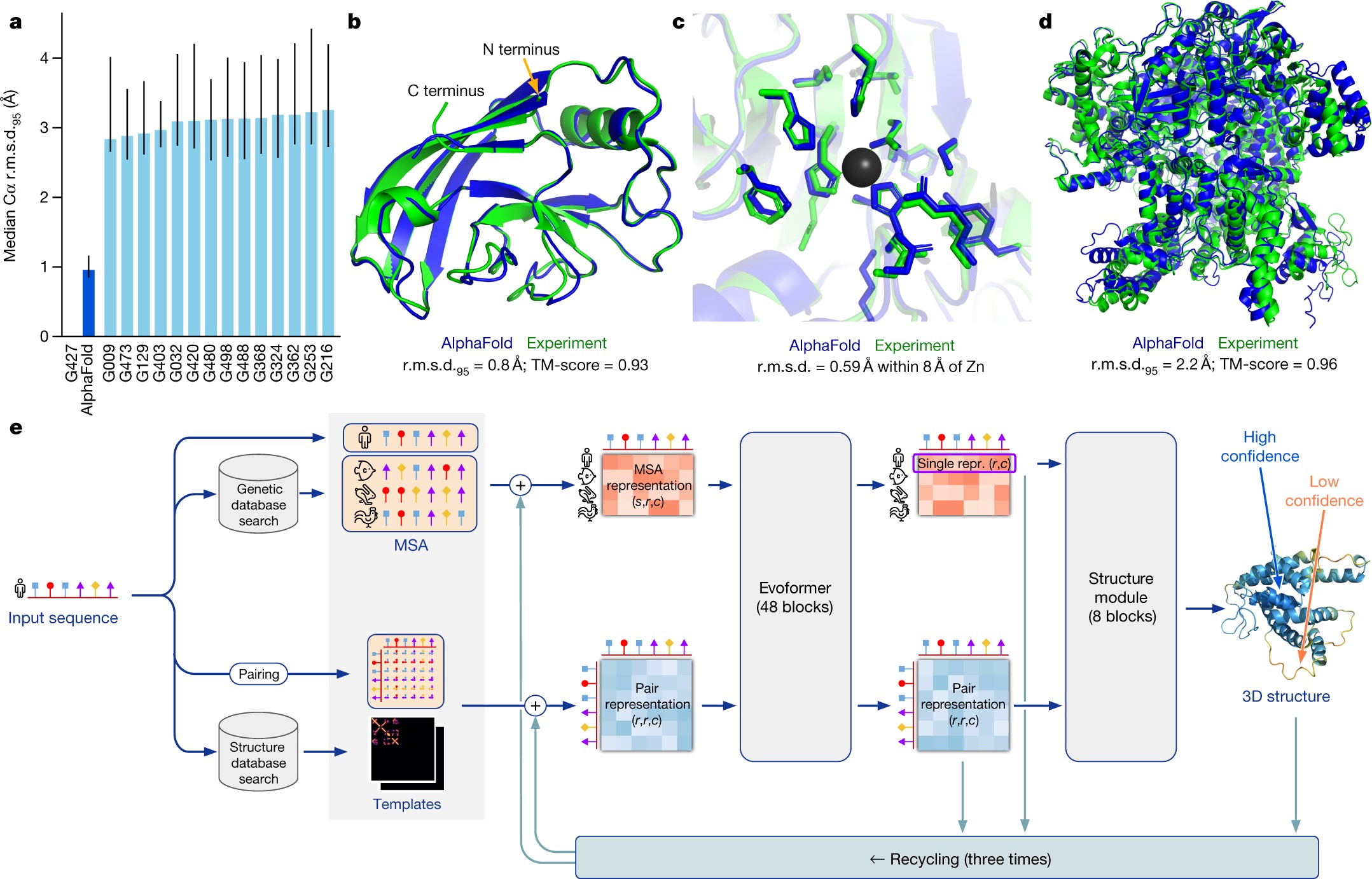
The algorithm takes several inputs, including the primary sequence of the protein and sequences of evolutionarily related proteins. These related sequences are formatted as a Multiple Sequence Alignment (MSA) created using tools like jackhmmer and HHBlits. Where available, the algorithm also uses 3D atom coordinates of homologous structures (templates). The search processes for both MSA and templates are optimized for high recall.
The Big Fantastic Database (BFD), a custom-built and publicly released database, is a crucial resource. BFD contains 65,983,866 families, represented as MSAs and Hidden Markov Models (HMMs), covering over two billion protein sequences. This database significantly expands the range of proteins that can be accurately modeled.
BFD’s creation involved three key steps: protein sequence collection and clustering, representative protein sequence addition from Metaclust NR, and MSA computation using FAMSA, followed by HMM construction.
Public datasets used in this study include a copy of the PDB downloaded on 28 August 2019 for training, and a copy downloaded on 14 May 2020 for finding template structures. MSA lookup used Uniref90 v.2020_01, BFD, Uniclust30 v.2018_08, and MGnify v.2018_12. Uniclust30 v.2018_08 was used for sequence distillation.
HHBlits and HHSearch (from hh-suite v.3.0-beta.3) were employed for MSA search on BFD + Uniclust30 and template search against PDB70. Jackhmmer (from HMMER3) was used for MSA search on Uniref90 and clustered MGnify. Structure relaxation utilized OpenMM v.7.3.1 with the Amber99sb force field. TensorFlow, Sonnet, NumPy, Python, and Colab were used for neural network construction, execution, and analyses.
Removing BFD reduces mean accuracy by 0.4 GDT, Mgnify by 0.7 GDT, and both by 6.1 GDT. Targets may have very small changes in accuracy. But a few outliers had very large (20+ GDT) differences. The depth of the MSA is unimportant until around 30 sequences, when the MSA size effects become quite large. The metagenomics databases are very important for target classes that are poorly represented in UniRef.
Training and Prediction
The model is trained using structures from the PDB with a maximum release date of 30 April 2018. Chains are sampled in inverse proportion to cluster size. It is randomly cropped to 256 residues and assembled into batches of size 128. The model is trained on Tensor Processing Unit (TPU) v3. Training continues until convergence (around 10 million samples). It is further fine-tuned using longer crops of 384 residues, larger MSA stack and reduced learning rate (see Supplementary Methods 1.11 for the exact configuration). The initial training stage takes about 1 week. The fine-tuning stage takes approximately 4 additional days.
The network is supervised by the FAPE loss and auxiliary losses. The final pair representation is linearly projected to a binned distance distribution (distogram) prediction, scored with a cross-entropy loss. Random masking on the input MSAs requires the network to reconstruct the masked regions using a BERT-like loss. The output single representations of the structure module predict binned per-residue lDDT-Cα values. An auxiliary side-chain loss is used during training, and an auxiliary structure violation loss during fine-tuning.
A final model with identical hyperparameters sampled 75% of the time from the Uniclust prediction set, with sub-sampled MSAs, and 25% of the time from the clustered PDB set.
Five different models using different random seeds, some with templates and some without, encourage diversity in the predictions. These models were fine-tuned after CASP14 to add a pTM prediction objective (Supplementary Methods 1.9.7) and use the obtained models.
Inference Regimen
The trained models are inferred and use the predicted confidence score to select the best model per target.
The trunk of the network is run multiple times with different random choices for the MSA cluster centres. Representative timings for the neural network using a single model on V100 GPU are 4.8 min with 256 residues, 9.2 min with 384 residues and 18 h at 2,500 residues. This open-source code is notably faster than the version we ran in CASP14 as we now use the XLA compiler.
The network without ensembling is very close or equal to the accuracy with ensembling and we turn off ensembling for most inference. Without ensembling, the network is 8× faster and the representative timings for a single model are 0.6 min with 256 residues, 1.1 min with 384 residues and 2.1 h with 2,500 residues.
For a V100 with 16 GB of memory, the structure of proteins up to around 1,300 residues can be predicted. The memory usage is approximately quadratic in the number of residues, so a 2,500-residue protein involves using unified memory. A single V100 is used for computation on a 2,500-residue protein but we requested four GPUs to have sufficient memory.
Searching genetic sequence databases to prepare inputs and final relaxation of the structures take additional central processing unit (CPU) time.
Evaluating Performance
The predicted structure is compared to the true structure from the PDB in terms of lDDT metric. The distances are computed between all heavy atoms (lDDT) or only the Cα atoms to measure the backbone accuracy (lDDT-Cα). Domain accuracies in CASP are reported as GDT and the TM-score is used as a full chain global superposition metric.
Accuracies are also reported using the r.m.s.d.95 (Cα r.m.s.d. at 95% coverage). The r.m.s.d. of the atoms chosen for the final iterations is the r.m.s.d.95.
Test Set of Recent PDB Sequences
For evaluation on recent PDB sequences, a copy of the PDB downloaded 15 February 2021 was used. Structures were filtered to those with a release date after 30 April 2018. Chains were further filtered to remove single amino acid sequences, sequences with an ambiguous chemical component, and exact duplicates. Structures with less than 16 resolved residues, with unknown residues or solved by NMR methods were removed. The chain with the highest resolution was selected from each cluster in the PDB 40% sequence clustering of the data. Sequences for which fewer than 80 amino acids had the alpha carbon resolved and chains with more than 1,400 residues were removed. The final dataset contained 10,795 protein sequences.
The MSA depth analysis was based on computing the normalized number of effective sequences (Neff) for each position of a query sequence. Per-residue Neff values were obtained by counting the number of non-gap residues in the MSA and weighting the sequences using the Neff scheme with a threshold of 80% sequence identity.
Legal Considerations and Kohl Implementations
While the core AlphaFold algorithm is open-source, its use may be subject to certain licensing terms and conditions. Researchers and developers should carefully review these terms before deploying the algorithm in commercial or non-commercial settings. Kohl refers to a specific implementation or adaptation of the AlphaFold algorithm, and details about its development and usage can be found in relevant research publications and documentation.
Conclusion
AlphaFold represents a significant advancement in protein structure prediction. By understanding its core components, data sources, and training methodologies, researchers can leverage this powerful tool to accelerate discoveries in biology and medicine. This guide provides a foundational understanding of AlphaFold, encouraging further exploration and innovation in the field.