A Complete Guide to XGBoost: Parameters, Tuning, and Practical Examples

XGBoost (Extreme Gradient Boosting) has become a go-to algorithm for data scientists aiming for top performance in predictive modeling. Its ability to handle complex data irregularities and leverage parallel computation for efficient training makes it a powerful tool. This article provides A Complete Guide To Xgboost, focusing on parameter tuning and practical application using Python. Whether you’re new to XGBoost or looking to refine your skills, this guide will provide valuable insights.

What is XGBoost?

XGBoost is a highly effective gradient boosting algorithm celebrated for its speed and accuracy in machine learning. While XGBoost simplifies the machine learning model creation, optimizing its performance can be challenging due to its intricate parameter tuning. Choosing the correct parameters and determining their ideal values are essential for achieving optimal results. This process can be daunting, especially when deciding which parameters deserve the most attention. This guide provides the practical knowledge necessary to fine-tune your XGBoost models and achieve the best possible outcomes.

XGBoost builds upon the foundations of the Gradient Boosting Machine (GBM). If you’re familiar with GBM, understanding XGBoost parameters will be much easier.

For instance, in HR analytics, XGBoost can revolutionize operations by providing predictive insights. While HR departments have used analytics for years, manual data collection and analysis can be inefficient. Machine learning, especially predictive analytics powered by XGBoost, can identify employees with high promotion potential, improving HR efficiency and overall results.

Advantages of XGBoost

XGBoost offers several advantages that contribute to its popularity and effectiveness:

Regularization

Unlike standard GBM implementations, XGBoost incorporates regularization techniques, like L1 and L2 regularization, effectively reducing overfitting. This makes XGBoost known as a ‘regularized boosting’ technique.

Parallel Processing

XGBoost leverages parallel processing, making it significantly faster than GBM. Even though boosting is inherently a sequential process (each tree depends on the previous one), XGBoost parallelizes the creation of individual trees by utilizing all available cores.

High Flexibility

XGBoost allows users to define custom optimization objectives and evaluation criteria. This flexibility enables tailoring the model to specific problem requirements.

Handling Missing Values

XGBoost has a built-in mechanism for handling missing values. By allowing the user to specify a distinct value for missing data, XGBoost can learn the optimal path for these values during the tree-building process.

Tree Pruning

Unlike GBM, which stops splitting a node when it encounters a negative loss, XGBoost grows trees to the specified max_depth and then prunes them backward. This approach helps XGBoost overcome the limitations of a greedy algorithm and potentially capture splits that, while initially appearing negative, lead to overall positive gains deeper in the tree.

Built-in Cross-Validation

XGBoost enables cross-validation at each boosting iteration, allowing for easy determination of the optimal number of boosting iterations in a single run.

Continue on the Existing Model

Users can continue training an XGBoost model from its last iteration of the previous run. This is particularly useful in applications where retraining is necessary due to new data or changes in the problem.

What are XGBoost Parameters?

XGBoost parameters are divided into three main categories:

• General Parameters: Control overall functioning.
• Booster Parameters: Guide the individual boosters (trees/regression) at each step.
• Learning Task Parameters: Guide the optimization performed.

General Parameters

These parameters define the global configuration of XGBoost:

• booster [default=gbtree]
  • Specifies the type of model to run at each iteration.
    • gbtree: tree-based models
    • gblinear: linear models
• silent [default=0]
  • Controls verbosity. Set to 1 to suppress running messages.
• nthread [default=Maximum number of threads available]
  • Sets the number of threads for parallel processing. If not specified, XGBoost will automatically detect and use all available cores.

Booster Parameters

These parameters control the individual trees within the ensemble. It’s important to note that while there are two types of boosters, the tree booster generally outperforms the linear booster and is more commonly used.

Parameter	Description	Typical Values
eta	Learning rate, analogous to the learning rate in GBM.	0.01-0.2
min_child_weight	Minimum sum of weights of observations required in a child node.	Tuned with CV
max_depth	Maximum depth of a tree. Controls overfitting.	3-10
max_leaf_nodes	The maximum number of terminal nodes or leaves in a tree.	N/A
gamma	Minimum loss reduction required to make a split.	Tuned based on loss function
max_delta_step	Constrains each tree’s weight estimation.	Rarely needed
subsample	Fraction of observations to be randomly sampled for each tree.	0.5-1
colsample_bytree	Fraction of columns to be randomly sampled for each tree.	0.5-1
colsample_bylevel	Subsample ratio of columns for each split, in each level.	Rarely used
lambda	L2 regularization term on weights (analogous to Ridge regression). Reduces overfitting.	Explore
alpha	L1 regularization term on weights (analogous to Lasso regression). Useful for high dimensionality.	Use if needed
scale_pos_weight	Used in case of high-class imbalance for faster convergence.	> 0

Learning Task Parameters

These parameters define the optimization objective and the metric used for evaluation:

• objective [default=reg:linear]
  • Specifies the loss function to be minimized.
    • binary:logistic: Logistic regression for binary classification, returns predicted probability.
    • multi:softmax: Multiclass classification using the softmax objective, returns predicted class. Requires setting num_class.
    • multi:softprob: Similar to softmax, but returns predicted probability for each class.
• eval_metric [default=rmse for regression, error for classification]
  • Evaluation metric for validation data.
    • rmse: Root mean square error
    • mae: Mean absolute error
    • logloss: Negative log-likelihood
    • error: Binary classification error rate (0.5 threshold)
    • merror: Multiclass classification error rate
    • mlogloss: Multiclass logloss
    • auc: Area under the curve
• seed [default=0]
  • Random number seed for reproducible results and parameter tuning.

If you’re familiar with Scikit-Learn, the XGBoost module in Python offers an sklearn wrapper called XGBClassifier. It uses the sklearn-style naming convention:

• eta –> learning_rate
• lambda –> reg_lambda
• alpha –> reg_alpha

The n_estimators parameter in GBM is equivalent to num_boosting_rounds when calling the fit function in the standard XGBoost implementation.

XGBoost Parameter Tuning with Example

To illustrate parameter tuning, we’ll use a dataset from a past Data Hackathon, similar to the example used in the GBM article.

The following steps are performed to prepare the data:

• Dropped the city variable due to too many categories.
• Converted DOB to Age.
• Created EMI_Loan_Submitted_Missing (1 if missing, 0 otherwise).
• Dropped EmployerName due to too many categories.
• Imputed Existing_EMI with 0 (median).
• Created Interest_Rate_Missing (1 if missing, 0 otherwise).
• Dropped Lead_Creation_Date.
• Imputed Loan_Amount_Applied and Loan_Tenure_Applied with median values.
• Created Loan_Amount_Submitted_Missing and Loan_Tenure_Submitted_Missing (1 if missing, 0 otherwise).
• Dropped LoggedIn and Salary_Account.
• Created Processing_Fee_Missing (1 if missing, 0 otherwise).
• Kept the top 2 values of Source as is and combined all others into a different category.
• Performed numerical and one-hot encoding.

Let’s begin by importing the necessary libraries and loading the data.

#Import libraries
import pandas as pd
import numpy as np
import xgboost as xgb
from xgboost.sklearn import XGBClassifier
from sklearn import metrics
#Additional scklearn functions
from sklearn.model_selection import GridSearchCV
import matplotlib.pylab as plt
from matplotlib.pylab import rcParams
rcParams['figure.figsize'] = 12, 4

train = pd.read_csv('Train_Modified.csv', encoding='ISO-8859–1')
target = 'Disbursed'
IDcol = 'ID'
print("There will be no output for this particular block of code")

We import two forms of XGBoost:

• xgb: The direct XGBoost library, which includes specific functions like cv.
• XGBClassifier: An sklearn wrapper for XGBoost, allowing the use of sklearn’s Grid Search with parallel processing.

Next, we define a function to create XGBoost models and perform cross-validation:

def modelfit(alg, dtrain, predictors,useTrainCV=True, cv_folds=5, early_stopping_rounds=50):
    if useTrainCV:
        xgb_param = alg.get_xgb_params()
        xgtrain = xgb.DMatrix(dtrain[predictors].values, label=dtrain[target].values)
        cvresult = xgb.cv(xgb_param, xgtrain, num_boost_round=alg.get_params()['n_estimators'], nfold=cv_folds,
                            metrics='auc', early_stopping_rounds=early_stopping_rounds, show_progress=False)
        alg.set_params(n_estimators=cvresult.shape[0])

    #Fit the algorithm on the data
    alg.fit(dtrain[predictors], dtrain['Disbursed'],eval_metric='auc')

    #Predict training set:
    dtrain_predictions = alg.predict(dtrain[predictors])
    dtrain_predprob = alg.predict_proba(dtrain[predictors])[:,1]

    #Print model report:
    print "nModel Report"
    print "Accuracy : %.4g" % metrics.accuracy_score(dtrain['Disbursed'].values, dtrain_predictions)
    print "AUC Score (Train): %f" % metrics.roc_auc_score(dtrain['Disbursed'], dtrain_predprob)

    feat_imp = pd.Series(alg.booster().get_fscore()).sort_values(ascending=False)
    feat_imp.plot(kind='bar', title='Feature Importances')
    plt.ylabel('Feature Importance Score')

General Approach for XGBoost Parameter Tuning

We’ll use a similar approach to GBM:

1. Choose a High Learning Rate: Start with a learning rate of 0.1 (or between 0.05 and 0.3). Determine the optimal number of trees using XGBoost’s cv function.
2. Tune Tree-Specific Parameters: Tune max_depth, min_child_weight, gamma, subsample, and colsample_bytree.
3. Tune Regularization Parameters: Tune lambda and alpha to reduce model complexity.
4. Lower the Learning Rate: Reduce the learning rate and re-optimize the number of trees.

Step 1: Fix Learning Rate and Number of Estimators

We start by setting initial values for the parameters:

• max_depth = 5
• min_child_weight = 1
• gamma = 0
• subsample, colsample_bytree = 0.8
• scale_pos_weight = 1

Let’s use a learning rate of 0.1 and find the optimal number of trees:

#Choose all predictors except target & IDcols
predictors = [x for x in train.columns if x not in [target, IDcol]]
xgb1 = XGBClassifier(
    learning_rate =0.1,
    n_estimators=1000,
    max_depth=5,
    min_child_weight=1,
    gamma=0,
    subsample=0.8,
    colsample_bytree=0.8,
    objective= 'binary:logistic',
    nthread=4,
    scale_pos_weight=1,
    seed=27
)
modelfit(xgb1, train, predictors)

This results in an optimal estimator count of 140 for a learning rate of 0.1.

Step 2: Tune max_depth and min_child_weight

These parameters significantly impact the model. We’ll start with wider ranges and then refine them.

param_test1 = {
    'max_depth':range(3,10,2),
    'min_child_weight':range(1,6,2)
}
gsearch1 = GridSearchCV(
    estimator = XGBClassifier(
        learning_rate =0.1,
        n_estimators=140,
        max_depth=5,
        min_child_weight=1,
        gamma=0,
        subsample=0.8,
        colsample_bytree=0.8,
        objective= 'binary:logistic',
        nthread=4,
        scale_pos_weight=1,
        seed=27
    ),
    param_grid = param_test1,
    scoring='roc_auc',
    n_jobs=4,
    iid=False,
    cv=5
)
gsearch1.fit(train[predictors],train[target])
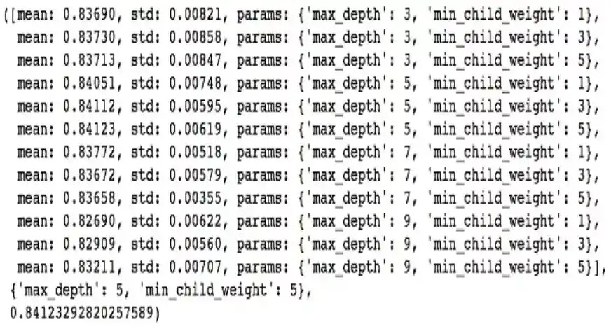
print('Grid scores:', gsearch1.cv_results_['mean_test_score'])
print('Best parameters:', gsearch1.best_params_)
print('Best score:', gsearch1.best_score_)

The ideal values are 5 for max_depth and 5 for min_child_weight. Let’s further refine the search:

param_test2 = {
    'max_depth':[4,5,6],
    'min_child_weight':[4,5,6]
}
gsearch2 = GridSearchCV(
    estimator = XGBClassifier(
        learning_rate=0.1,
        n_estimators=140,
        max_depth=5,
        min_child_weight=2,
        gamma=0,
        subsample=0.8,
        colsample_bytree=0.8,
        objective= 'binary:logistic',
        nthread=4,
        scale_pos_weight=1,
        seed=27
    ),
    param_grid = param_test2,
    scoring='roc_auc',
    n_jobs=4,
    iid=False,
    cv=5
)
gsearch2.fit(train[predictors],train[target])
print('Grid scores:', gsearch2.cv_results_['mean_test_score'])
print('Best parameters:', gsearch2.best_params_)
print('Best score:', gsearch2.best_score_)

Now, the optimum values are 4 for max_depth and 6 for min_child_weight.

Step 3: Tune gamma

Let’s tune the gamma value using the tuned parameters:

param_test3 = {
    'gamma':[i/10.0 for i in range(0,5)]
}
gsearch3 = GridSearchCV(
    estimator = XGBClassifier(
        learning_rate =0.1,
        n_estimators=140,
        max_depth=4,
        min_child_weight=6,
        gamma=0,
        subsample=0.8,
        colsample_bytree=0.8,
        objective= 'binary:logistic',
        nthread=4,
        scale_pos_weight=1,
        seed=27
    ),
    param_grid = param_test3,
    scoring='roc_auc',
    n_jobs=4,
    iid=False,
    cv=5
)
gsearch3.fit(train[predictors],train[target])
print('Grid scores:', gsearch3.cv_results_['mean_test_score'])
print('Best parameters:', gsearch3.best_params_)
print('Best score:', gsearch3.best_score_)

The original value of gamma, 0, remains the optimum. Before proceeding, re-calibrate the number of boosting rounds:

xgb2 = XGBClassifier(
    learning_rate =0.1,
    n_estimators=1000,
    max_depth=4,
    min_child_weight=6,
    gamma=0,
    subsample=0.8,
    colsample_bytree=0.8,
    objective= 'binary:logistic',
    nthread=4,
    scale_pos_weight=1,
    seed=27
)
modelfit(xgb2, train, predictors)

The final parameters are:

• max_depth: 4
• min_child_weight: 6
• gamma: 0

Step 4: Tune subsample and colsample_bytree

Next, we experiment with different values for subsample and colsample_bytree:

param_test4 = {
    'subsample':[i/10.0 for i in range(6,10)],
    'colsample_bytree':[i/10.0 for i in range(6,10)]
}
gsearch4 = GridSearchCV(
    estimator = XGBClassifier(
        learning_rate =0.1,
        n_estimators=177,
        max_depth=4,
        min_child_weight=6,
        gamma=0,
        subsample=0.8,
        colsample_bytree=0.8,
        objective= 'binary:logistic',
        nthread=4,
        scale_pos_weight=1,
        seed=27
    ),
    param_grid = param_test4,
    scoring='roc_auc',
    n_jobs=4,
    iid=False,
    cv=5
)
gsearch4.fit(train[predictors],train[target])
print('Grid scores:', gsearch4.cv_results_['mean_test_score'])
print('Best parameters:', gsearch4.best_params_)
print('Best score:', gsearch4.best_score_)

Here, 0.8 is the optimum value for both subsample and colsample_bytree.

Step 5: Tuning Regularization Parameters

We apply regularization to reduce overfitting. Let’s tune the reg_alpha value:

param_test6 = {
    'reg_alpha':[1e-5, 1e-2, 0.1, 1, 100]
}
gsearch6 = GridSearchCV(
    estimator = XGBClassifier(
        learning_rate =0.1,
        n_estimators=177,
        max_depth=4,
        min_child_weight=6,
        gamma=0.1,
        subsample=0.8,
        colsample_bytree=0.8,
        objective= 'binary:logistic',
        nthread=4,
        scale_pos_weight=1,
        seed=27
    ),
    param_grid = param_test6,
    scoring='roc_auc',
    n_jobs=4,
    iid=False,
    cv=5
)
gsearch6.fit(train[predictors],train[target])
print('Grid scores:', gsearch6.cv_results_['mean_test_score'])
print('Best parameters:', gsearch6.best_params_)
print('Best score:', gsearch6.best_score_)

Refining the search around 0.01:

param_test7 = {
    'reg_alpha':[0, 0.001, 0.005, 0.01, 0.05]
}
gsearch7 = GridSearchCV(
    estimator = XGBClassifier(
        learning_rate =0.1,
        n_estimators=177,
        max_depth=4,
        min_child_weight=6,
        gamma=0.1,
        subsample=0.8,
        colsample_bytree=0.8,
        objective= 'binary:logistic',
        nthread=4,
        scale_pos_weight=1,
        seed=27
    ),
    param_grid = param_test7,
    scoring='roc_auc',
    n_jobs=4,
    iid=False,
    cv=5
)
gsearch7.fit(train[predictors],train[target])
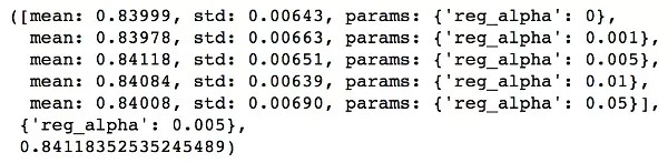
print('Grid scores:', gsearch7.cv_results_['mean_test_score'])
print('Best parameters:', gsearch7.best_params_)
print('Best score:', gsearch7.best_score_)

We apply this regularization in the model:

xgb3 = XGBClassifier(
    learning_rate =0.1,
    n_estimators=1000,
    max_depth=4,
    min_child_weight=6,
    gamma=0,
    subsample=0.8,
    colsample_bytree=0.8,
    reg_alpha=0.005,
    objective= 'binary:logistic',
    nthread=4,
    scale_pos_weight=1,
    seed=27
)
modelfit(xgb3, train, predictors)

Step 6: Reducing the Learning Rate

Finally, we lower the learning rate and increase the number of trees:

xgb4 = XGBClassifier(
    learning_rate =0.01,
    n_estimators=5000,
    max_depth=4,
    min_child_weight=6,
    gamma=0,
    subsample=0.8,
    colsample_bytree=0.8,
    reg_alpha=0.005,
    objective= 'binary:logistic',
    nthread=4,
    scale_pos_weight=1,
    seed=27
)
modelfit(xgb4, train, predictors)

Conclusion

This guide provides a comprehensive overview of XGBoost parameters, tuning techniques, and practical examples. By systematically tuning these parameters, you can significantly improve your model’s performance. Remember to focus on feature engineering, creating ensembles of models, and stacking for even greater gains. The XGBoost algorithm is a powerful tool used in machine learning. The XGBoost classifier helps improve predictions by using an XGBoost model.

Key Takeaways

• XGBoost is a powerful machine-learning algorithm, known for its speed and accuracy.
• Consider different parameters and their values when implementing an XGBoost model.
• XGBoost hyperparameters model requires parameter tuning to improve and fully leverage its advantages over other algorithms.

Frequently Asked Questions

Q1. What parameters should you use for XGBoost?

A. The choice of XGBoost parameters depends on the specific task. Commonly adjusted parameters include learning rate (eta), maximum tree depth (max_depth), and minimum child weight (min_child_weight).

Q2. What does the ‘N_estimators’ parameter signify in XGBoost?

A. The ‘n_estimators’ parameter in XGBoost determines the number of boosting rounds or trees to build. It directly impacts the model’s complexity and should be tuned for optimal performance.

Q3. How do you define a hyperparameter in XGBoost?

A. In XGBoost, a hyperparameter is a preset setting that isn’t learned from the data but must be configured before training. Examples include the learning rate, tree depth, and regularization parameters.

Q4. What purpose do regularization parameters serve in XGBoost?

A. XGBoost provides L1 and L2 regularization terms using the ‘alpha’ and ‘lambda’ parameters, respectively. These parameters prevent overfitting by adding penalty terms to the objective function during training.