A Comprehensive Guide to Convolutional Neural Networks: Towards Data Science

Convolutional Neural Networks (CNNs), also known as ConvNets, are a specialized type of neural network particularly effective at processing data with a grid-like structure, most notably images. Understanding how CNNs work is crucial in the field of computer vision and deep learning. This guide provides a detailed overview of CNNs, their architecture, and their applications, with a focus on delivering insights beyond a basic introduction, drawing inspiration from resources like towardsdatascience.com.

Understanding the Basics

A digital image, at its core, is a numerical representation of visual information. It’s essentially a grid of pixels, each holding a value that determines its brightness and color.

Figure 1: A digital image represented as a grid of pixels, where each pixel’s value determines its color and brightness.

The human brain rapidly processes visual information, with neurons responding to specific regions of the visual field. CNNs mimic this process, with each neuron focusing on a localized area known as its receptive field. This localized processing, combined across layers, allows CNNs to identify simple patterns initially (edges, corners) and progressively more complex patterns (objects, faces) further down the line. This makes them a powerful tool for enabling computers to “see”.

CNN Architecture: A Layered Approach

A typical CNN architecture consists of three fundamental layer types: convolutional layers, pooling layers, and fully connected layers. Each layer plays a distinct role in feature extraction and classification.

Figure 2: Illustrative representation of a Convolutional Neural Network (CNN) architecture, showcasing the typical arrangement of convolutional, pooling, and fully connected layers.

Convolutional Layer: The Feature Extractor

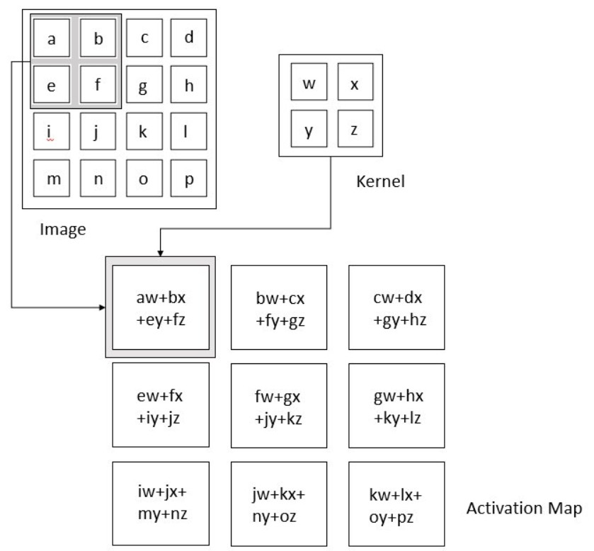
The convolutional layer is the engine of a CNN, responsible for the bulk of the computational effort. It operates by performing a dot product between a kernel (a small matrix of learnable parameters) and a localized region of the input data (the receptive field).

This kernel, smaller than the entire input image but extending through all its channels (e.g., RGB), slides across the image, generating a feature map. The size of the “slide” is called the stride. This process essentially identifies specific features present in the image.

Animated illustration depicting the convolution operation, where a kernel slides across the image to produce an activation map, highlighting the response of the kernel at each spatial position.

The output volume size (Wout x Wout x Dout) of a convolutional layer can be calculated using the following formula:

Wout = (W – F + 2P) / S + 1

Where:

• W is the input size
• F is the kernel size
• P is the padding
• S is the stride
• Dout is the number of kernels

The convolution operation is motivated by three key ideas:

• Sparse Interactions: Instead of every neuron connecting to every input (as in traditional neural networks), each neuron in a convolutional layer only connects to a local region of the input. This reduces the number of parameters and computational cost.
• Parameter Sharing: The same kernel (set of weights) is used across the entire input image to detect a specific feature. This significantly reduces the number of parameters and allows the network to learn features that are invariant to their location in the image.
• Equivariant Representation: Convolutional layers are equivariant to translation. This means that if the input image is shifted, the feature map will also be shifted by the same amount.

Pooling Layer: Downsampling and Generalization

The pooling layer simplifies the representation by reducing its spatial dimensions. It aggregates the outputs of neuron clusters at one layer into a single neuron in the next layer. This downsampling helps to reduce the computational load and makes the network more robust to variations in the input.

Common pooling functions include average pooling, L2-norm pooling, and max pooling. Max pooling, which selects the maximum value from each region, is the most widely used.

Figure 4: Illustration of the pooling operation. Max pooling, shown here, selects the largest value from each region of the feature map.

The output volume size (Wout x Wout x D) of a pooling layer can be calculated using the following formula:

Wout = (W – F) / S + 1

Where:

• W is the input size
• F is the kernel size
• S is the stride
• D is the depth

Pooling layers introduce a degree of translation invariance, meaning that the network becomes less sensitive to the precise location of features in the input image.

Fully Connected Layer: Classification

The fully connected (FC) layer is the final stage in a CNN. Neurons in this layer have full connections to all activations in the previous layer, just like in a traditional multilayer perceptron. The flattened output from the previous layers is fed into one or more fully connected layers.

The FC layer learns to map the features extracted by the convolutional and pooling layers to the final output classes.

Non-Linearity Layers: Adding Complexity

Because convolution is a linear operation and images are inherently non-linear, non-linearity layers are crucial. These layers introduce non-linear activation functions, allowing the network to learn complex patterns. Common non-linearities include:

• Sigmoid: Squashes values between 0 and 1. However, it suffers from vanishing gradients, especially in deep networks.
• Tanh: Similar to sigmoid but squashes values between -1 and 1. It addresses the non-zero centered output issue of sigmoid but still suffers from vanishing gradients.
• ReLU (Rectified Linear Unit): Activates a neuron only if the input is above zero. ReLU is computationally efficient and helps to alleviate the vanishing gradient problem.

Designing a CNN: A Practical Example

Let’s consider a practical example using the Fashion-MNIST dataset, which contains 60,000 training images and 10,000 test images of Zalando’s article images. Each image is 28×28 grayscale and belongs to one of 10 classes.

A possible CNN architecture for this dataset could be:

INPUT -> CONV1 -> BATCH NORM -> ReLU -> POOL1 -> CONV2 -> BATCH NORM -> ReLU -> POOL2 -> FC LAYER -> RESULT

We can define the constraints for Conv1, Pool1, Conv2, and Pool2 layers. For example, the Conv1 layer can have a 5×5 kernel with a stride of 1 and padding of 2. Similarly, we can define constraints for the remaining layers.

The code snippet defining such a convnet in PyTorch might look like this:

import torch.nn as nn

class ConvNet(nn.Module):
    def __init__(self):
        super(ConvNet, self).__init__()
        self.conv1 = nn.Conv2d(in_channels=1, out_channels=16, kernel_size=5, stride=1, padding=2)
        self.batch1 = nn.BatchNorm2d(16)
        self.relu1 = nn.ReLU()
        self.pool1 = nn.MaxPool2d(kernel_size=2)
        self.conv2 = nn.Conv2d(in_channels=16, out_channels=32, kernel_size=5, stride=1, padding=2)
        self.batch2 = nn.BatchNorm2d(32)
        self.relu2 = nn.ReLU()
        self.pool2 = nn.MaxPool2d(kernel_size=2)
        self.fc = nn.Linear(32 * 7 * 7, 10)

    def forward(self, x):
        out = self.conv1(x)
        out = self.batch1(out)
        out = self.relu1(out)
        out = self.pool1(out)
        out = self.conv2(out)
        out = self.batch2(out)
        out = self.relu2(out)
        out = self.pool2(out)
        out = out.view(out.size(0), -1)
        out = self.fc(out)
        return out

Batch normalization, used in this network, helps stabilize training by normalizing the activations of each layer. Training typically involves using a loss function (like cross-entropy) and an optimizer (like Adam) to adjust the network’s weights based on the training data.

Applications of CNNs: Seeing is Believing

CNNs are the driving force behind many real-world applications:

1. Object Detection: CNN-based models like R-CNN, Fast R-CNN, and Faster R-CNN are crucial components in autonomous vehicles, facial detection systems, and more.
2. Semantic Segmentation: CNNs enable the labeling of each pixel in an image, allowing for a deeper understanding of the scene.
3. Image Captioning: CNNs, in combination with recurrent neural networks (RNNs), can generate descriptive captions for images and videos.

Conclusion: The Power of Convolution

Convolutional Neural Networks have revolutionized the field of computer vision, providing powerful tools for image recognition, object detection, and other visual tasks. By understanding the fundamental concepts and architecture of CNNs, you can leverage their capabilities to solve a wide range of real-world problems. As research continues, CNNs will undoubtedly play an even greater role in shaping the future of artificial intelligence.

References

1. Deep Learning by Ian Goodfellow, Yoshua Bengio and Aaron Courville published by MIT Press, 2016
2. Stanford University’s Course – CS231n: Convolutional Neural Network for Visual Recognition by Prof. Fei-Fei Li, Justin Johnson, Serena Yeung
3. https://datascience.stackexchange.com/questions/14349/difference-of-activation-functions-in-neural-networks-in-general
4. https://www.codementor.io/james_aka_yale/convolutional-neural-networks-the-biologically-inspired-model-iq6s48zms
5. https://searchenterpriseai.techtarget.com/definition/convolutional-neural-network