Causal modeling offers a powerful framework for representing hypothesized relationships within complex systems, providing a structured approach to understanding cause-and-effect (Long, 1983). Building upon the foundation laid in Part I, which focused on the conceptual underpinnings and construction of causal models, this second part serves as a consumer’s guide to causal modeling part ii, delving into the essential terminology and methods for evaluating model testing. Using an example from previous research (Youngblut, 1992), we will clarify the concepts to help in your understanding.
Essential Terminology in Causal Modeling
Understanding the language of causal modeling is crucial for interpreting research findings. Several key terms (see Table 1) are commonly used, and their definitions are essential for any consumer of research employing these techniques.
| Term | Definition |
|---|---|
| Latent variable | Theoretical concept or construct; not directly measured |
| Empirical indicator | Measured variable, e.g., score on a scale, number of heart beats per minute, number of days hospitalized |
| Exogenous variable | Latent variable that has arrows pointing away from it; can function only as an independent variable |
| Endogenous variable | Latent variable that has arrows pointing toward it; can also have arrows pointing away from it; functions as a dependent variable and possibly as an independent variable |
| Recursive model | All arrows between latent variables point in the same direction; no feedback loops |
| Nonrecursive model | Contains feedback loops; causal flow can go in both directions |
| Path | Arrow between two latent variables |
| Coefficient | Number that indicates the strength of the influence represented by the path |
| Free parameter | Characteristic of the population that will be estimated by the statistical program |
| Fit of the model | Degree to which the observed data are consistent with the proposed causal model |
Latent vs. Empirical Variables
Latent variables represent unobserved theoretical constructs, the core concepts we aim to understand. Empirical indicators, on the other hand, are the observable measurements collected in a study. In causal models, latent variables are typically depicted as circles, while empirical indicators are shown as rectangles. For example, consider a study examining the impact of maternal employment on child development.
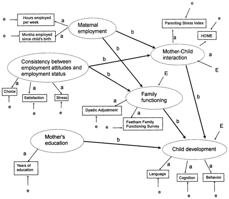 Causal model with empirical indicators
Here, Maternal Employment and Family Functioning are latent variables, abstract concepts that cannot be directly measured. Instead, we use empirical indicators such as “Hours Employed per Week” and “Months Employed Since Child’s Birth” for Maternal Employment, and “Dyadic Adjustment” and “Feetham Family Functioning Survey” scores for Family Functioning. The arrows connecting latent variables to their indicators point towards the indicators, reflecting the idea that the underlying concept influences the observed measurements, similar to factor analysis. The variable ‘a’ represents the Coefficient for strength of tie between empirical indicator and latent variable; ‘b’ represents the path coefficient for strength of effect of one latent variable on another; ‘e’ represents unexplained variance (error in measurement) in empirical indicator; and ‘E’ represents unexplained variance in an endogenous variable.
Exogenous vs. Endogenous Variables
Variables also differ in their role within the model. Exogenous variables are those whose causes are not explicitly modeled; they only have outgoing arrows. Endogenous variables, conversely, have incoming arrows, indicating that their causes are represented within the model.
In the example above, Maternal Employment, Consistency Between Employment Attitudes and Employment Status, and Mother’s Education are exogenous variables. Family Functioning, Mother-Child Interaction, and Child Development are endogenous variables. Family Functioning and Mother-Child Interaction are particularly interesting as they act as both independent and dependent variables within the model.
Recursive vs. Nonrecursive Models
Causal models can be further classified as either recursive or nonrecursive. Recursive models feature a unidirectional flow of causality, with no feedback loops. In contrast, nonrecursive models allow for reciprocal causation and feedback loops, representing situations where variables influence each other bidirectionally. Recursive models are generally simpler to analyze, while nonrecursive models require additional assumptions that can be difficult to justify.
Evaluating Model Fit: Assessing the Validity of the Hypothesized Relationships
A crucial step in causal modeling is evaluating how well the model fits the observed data. This involves assessing the degree to which the model’s predictions align with the actual data, indicating the validity of the hypothesized relationships.
Sample Size Considerations
The adequacy of the sample size is a critical factor in evaluating model fit. A parameter is a characteristic of the population (Sullivan & Feldman, 1979). The estimation is based on the number of free parameters in the model, which are population characteristics estimated by the statistical program. When a parameter is set to a specific value, it’s “fixed.” Otherwise, it’s “free” to vary with the sample data.
Each empirical indicator typically has two free parameters: the coefficient linking it to its latent variable (a in Figure 1) and an error term (e). An exception is a single indicator, where parameters are usually fixed. In Figure 1, Years of Education is a single indicator.
Counting the arrows between latent variables (b in Figure 1) also adds to the parameter count. Correlations between latent or observed variables, depicted by curved two-headed arrows, each count as one parameter. Finally, each endogenous variable has an error term (E in Figure 1).
According to Bentler and Chou (1988), a minimum of 5 to 10 cases per parameter is recommended for stable model testing. In the example, with 34 parameters, a minimum sample size of 170 is needed. A much smaller ratio may indicate unstable results that are less likely to hold up in future testing.
Assessing Statistical Significance and Fit Indices
While statistical significance is often a primary focus in other analyses, causal modeling prioritizes evaluating the overall fit of the model to the data. Programs like LISREL (Joreskog & Sorbom, 1986) and EQS (Bentler, 1989) provide a χ2 statistic, where a nonsignificant value indicates good fit. However, larger sample sizes (n ≥ 100) can inflate the χ2 statistic (Wheaton, 1987), making a nonsignificant value difficult to achieve.
Therefore, researchers often rely on other fit statistics, such as the Goodness-of-Fit Index (GFI) provided by LISREL, which ranges from 0 to 1 (Tanaka, 1993). Values of .90 and above generally indicate a good fit (Boyd, Frey, & Aaronson, 1988).
Model Trimming and Parameter Evaluation
The analysis process often involves “trimming the model” by removing nonsignificant paths and adding significant ones to achieve a better fit. Comparing the initial theoretical model with the final model reveals the extent of trimming. While publishing both models is ideal, space limitations may necessitate omitting the theoretical model. In such cases, the reader can often reconstruct the theoretical model by examining the literature review for implied relationships (Fawcett & Downs, 1991). Once a well-fitting model is obtained, the individual parameters are examined.
The path coefficients are evaluated for significance using a t-test, and their directions are compared to the expected directions. A model that fits the data but has many nonsignificant paths or paths with unexpected signs suggests that the relationships were not as theoretically specified. The coefficients between latent variables and empirical indicators should ideally fall between 0.50 and 1.0, indicating a strong tie. Values exceeding 1.0 often indicate a problem within the model. Finally, the unexplained variance (error) for each endogenous variable is evaluated. High unexplained variance suggests that the predictors do not adequately explain the outcomes, even if the model fits well overall.
Conclusion
Causal modeling provides a powerful tool for understanding complex relationships between theoretical constructs. However, it is crucial to interpret the results with caution. Achieving a good fit between the model and the data does not automatically validate all the hypothesized relationships. For researchers considering using causal modeling, the large sample sizes required can pose a significant challenge, resulting in more expensive and logistically complex studies. However, given the complex nature of many phenomena of interest, causal modeling remains an invaluable technique for advancing knowledge. This consumer’s guide to causal modeling part ii has equipped you with the knowledge to critically evaluate research employing these methods.
References
- Bentler, P. M. (1989). EQS structural equations program manual. BMDP Statistical Software.
- Bentler, P. M., & Chou, C. P. (1988). Practical issues in structural modeling. Sociological Methods & Research, 16(1), 78-117.
- Boyd, C. O., Frey, M. A., & Aaronson, L. S. (1988). Research utilization by nurses: Application of a causal model. Research in Nursing & Health, 11(5), 243-253.
- Fawcett, J., & Downs, F. S. (1991). How to conduct a thorough and relevant literature review. Journal of Obstetric, Gynecologic, & Neonatal Nursing, 20(1), 73-79.
- Joreskog, K. G., & Sorbom, D. (1986). LISREL VI user’s guide (4th ed.). Scientific Software.
- Long, J. S. (1983). Confirmatory factor analysis. Sage Publications.
- Nunnally, J. C. (1978). Psychometric theory. McGraw-Hill.
- Sullivan, D. S., & Feldman, J. J. (1979). Multiple indicators in survey and evaluation research. McGraw-Hill.
- Tanaka, J. S. (1993). Multifaceted conceptions of fit in structural equation models. In K. A. Bollen & J. S. Long (Eds.), Testing structural equation models (pp. 10-39). Sage Publications.
- Wheaton, B. (1987). Assessment of fit in overidentified models with latent variables. Sociological Methods & Research, 16(1), 118-154.
- Youngblut, J. M. (1992). A causal model of the effects of employment during pregnancy. Nursing Research, 41(5), 260-266.