Binding assays are crucial for quantifying interactions between molecules like proteins, small molecules, and nucleic acids. Proper design is essential to maximize the information gained from these assays, particularly in determining the affinity between reactants. This guide provides simple methods for optimizing binding experiments to yield comprehensive and quantitative data.
INTRODUCTION
In biochemistry and molecular biology, assessing molecular interactions is fundamental. Many published binding experiments are poorly designed, failing to extract maximum information from valuable reagents. A key deficiency is the omission of affinity measurements between reactants. Instead of simple “yes/no” answers, binding interactions should be quantified by affinity constants or affinity limits.
Two critical conditions for a successful binding experiment are achieving equilibrium during measurement and varying the concentration of at least one reactant. Common errors include disrupting equilibrium by separating reactants and products (e.g., in GST pull-down assays or immunoprecipitation) and neglecting to vary reactant concentrations. Journals should prioritize equilibrium experiments that measure equilibrium constants to prevent wasted resources.
This guide highlights experimental strategies for maximizing data from binding studies, emphasizing tools available in most laboratories. It details characteristics of well-designed assays that facilitate data analysis.
THE BASIC BINDING REACTION
Consider the reversible bimolecular binding reaction: molecule A binds to molecule B, forming complex AB:
A + B ⇆ AB
This reaction involves a forward reaction where A and B combine and a reverse reaction where AB dissociates into A and B. A 1:1 stoichiometry is typical in biological binding reactions.
The forward reaction A + B → AB is second order, with a rate defined as:
rate = k+ (A) (B)
Where:
- k+ is the second-order association rate constant (M−1s−1).
- (A) and (B) are the free concentrations of A and B.
Typical association rate constants for proteins range from 106 to 107 M−1s−1, limited by collision rates and interaction surface sizes. Smaller molecules diffuse faster, but this is balanced by smaller interaction surfaces.
The reverse reaction AB → A + B is first order, with a rate defined as:
rate = k− (AB)
Where:
- k− is the first-order dissociation rate constant (s−1).
- (AB) is the concentration of AB.
The dissociation rate constant indicates the probability of complex dissociation per unit time.
EQUILIBRIUM CONSTANTS
The equilibrium constant defines the affinity between molecules. At equilibrium, forward and reverse reaction rates are equal:
k+ (A) (B) = k− (AB)
The equilibrium constant (Keq) is the ratio of forward and reverse rate constants, or the ratio of product to reactant concentrations at equilibrium:
Keq = k+/k− = (AB) / (A)(B)
Keq has units of M−1, and its value directly correlates with affinity. A larger Keq indicates a stronger reaction and more complete conversion of reactants to product.
The dissociation equilibrium constant (Kd) is the reciprocal of Keq:
Kd = 1/Keq = (A)(B) / (AB)
Kd has units of M. Biologists prefer Kd because of its familiar units; a lower Kd indicates a stronger reaction.
Given the narrow range of association rate constants, the dissociation rate constant often dictates affinity. Micromolar Kd interactions have dissociation rate constants around 1 s−1 (half-life ~0.7 s), while nanomolar Kd interactions have dissociation rate constants around 0.001 s−1 (half-life >10 min).
The equilibrium constant relates to the free energy change (ΔG) for the reaction:
ΔG = -RT ln Keq
Where R is the gas constant, and T is the absolute temperature. Favorable reactions have large Keq and negative ΔG.
TWO STRATEGIES TO MEASURE EQUILIBRIUM CONSTANTS
Affinity can be measured using two main strategies:
- Equilibrium Experiment: Determine the reaction extent as a function of reactant concentration to derive the equilibrium constant.
- Kinetic Experiment: Determine forward and reverse reaction rates as a function of reactant concentration to calculate rate constants. The ratio of these yields the equilibrium constant.
Kinetic experiments provide more information, including both thermodynamic parameters and reaction dynamics. However, they often require more reagents and sophisticated assays. Equilibrium experiments only reveal affinity, providing no information on reaction rates.
EQUILIBRIUM BINDING EXPERIMENTS
This section outlines affinity measurement using equilibrium binding experiments. Practical advice for each step follows.
Consider the reversible binding reaction:
A + B ⇆ AB
Where:
Kd = (Afree)(Bfree) / (AB)
Assuming 1:1 stoichiometry, the task is to measure equilibrium concentrations of A, B, and AB across a range of reactant concentrations.
Five steps yield affinity:
- Develop a Sensitive Assay: Measure Aeq, Beq, or AB. (Afree) and (Bfree) refer to free A and B concentrations. Measuring one concentration is usually sufficient if total A and B concentrations are known.
- Design an Experiment: Use the lowest measurable concentrations of Afree, Bfree, or AB. Choose which reactant to fix and vary based on availability and ease of measurement. Using a low concentration of A simplifies the experiment and analysis.
- Set Up Reactions: Use a fixed, low concentration of total A and a wide range of B concentrations, spanning from below Kd to saturating levels. Pilot experiments can determine appropriate concentrations.
- Equilibrate: Allow reactions to reach equilibrium. Then, measure (Afree), (Bfree), or (AB) without disturbing equilibrium.
- Plot and Calculate: Plot AB concentration versus Bfree concentration and calculate Kd from the curve’s shape or the Bfree concentration at half-saturation.
ADVICE ON ASSAYS TO MEASURE BINDING REACTIONS
The assay for Afree, Bfree, or AB should be sensitive and simple. Afree and Bfree are the concentrations of free A and free B, not the total concentrations. The signal must be directly proportional to the concentration.
Chemical Assays
Calibrated chemical assays like gel electrophoresis, ELISA, and immunoblots can measure concentrations but must be done without altering the equilibrium.
Faults with Nonequilibrium Chemical Assays
Many assays prepare an equilibrium mixture but then separate products from reactants, causing dissociation. Examples include washing pelleted material, which eliminates reactants and drives dissociation. If affinity is low, dissociation is fast, making equilibrium concentration measurements impossible.
Equilibrium Chemical Assays
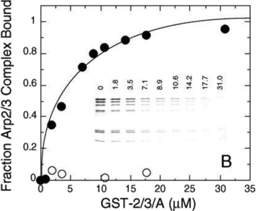
Separate products from reactants without disturbing equilibrium. If products have different sedimentation coefficients, pellet them, leaving reactants in the supernatant. For example, attach B to a bead and equilibrate with A. Pelleting separates bead-bound B and AB from free A. Measure free A in the supernatant to calculate AB.
To measure affinity, use a low, fixed concentration of A and vary the concentration of bead-bound B. Measuring the equilibrium concentration of AB as a function of Bfree (≈ total B) provides the data to calculate the affinity. Figure 1 illustrates a quantitative pull-down assay using gel electrophoresis and Coomassie staining to measure purified Arp2/3 complex concentration in the supernatant after equilibration with a GST-ligand bound to beads.
This strategy works with crude systems if a quantitative immunoblot or ELISA can measure free A. Titrate a crude extract containing low A with various concentrations of bead-bound B and measure free A in the supernatant.
If measuring AB in the pellet is necessary, minimize washing by using a glycerol or sucrose cushion. Brief washing (seconds) will minimize equilibrium disruption. Wash through a cushion by: 1) equilibrating, 2) pelleting through a cushion, 3) removing the supernatant and cushion, and 4) measuring bound B in the pellet.
The Advantages of Optical Assays
Optical assays offer speed and simplicity, enabling both equilibrium and kinetic measurements. Good optical assays measure one component’s concentration in equilibrium with the reaction’s other components.
Fluorescence Intensity
Differences in fluorescence intensity between product and reactants are the simplest optical assay. Intrinsic tryptophan fluorescence may change upon ligand binding. For instance, poly-L-proline binding increases profilin’s tryptophan fluorescence. While infrequent, check for intrinsic fluorescence signals.
Fluorescence Anisotropy
Measuring the fluorescence anisotropy of a fluorescently tagged reactant is universally useful. Anisotropy measures rotational diffusion; a larger product has a lower diffusion coefficient and higher anisotropy. For example, rhodamine-labeled WASp-VCA binding to Arp2/3 complex increases anisotropy. Use a low concentration of tagged molecule and titrate with untagged partner. Controls should include competition experiments with untagged molecules to account for any influence from the fluorescent dye.
Other Optical Assays
Fluorescence energy transfer requires tags on both reactants, increasing preparation and artifact chances. Light scattering can measure products that scatter more light than reactants, but signals are often noisy. Shorter wavelengths yield higher signals.
ADVICE ON EXPERIMENTAL DESIGN
Ideally, maintain a fixed total concentration of one reactant (e.g., A) lower than the Kd. A concentration ten-fold lower is suitable. This simplifies the experiment and data interpretation, as virtually all of the other reactant B remains free. The assay must be able to measure the concentration of free or bound A.
With low total A, determine the reaction extent over a wide range of B concentrations. When B is below the Kd, most B is free. At higher B concentrations, more AB forms, but A remains low enough that almost all B is free. Because Bfree ≈ Btotal, no compensation is needed for B bound to A.
If the assay lacks sensitivity for concentrations of A below Kd, use the lowest practical concentration of A. Compensate for B bound to A during data analysis.
ANALYSIS OF EQUILIBRIUM BINDING DATA
Plot AB concentration as a function of Bfree concentration to reveal the reaction’s extent. Include high B concentrations to saturate A and reach a plateau. Without this plateau, the amplitude of the reaction is unknown, preventing calculation of the equilibrium constant. Scatchard plots (bound/free vs. bound) were previously used, but are now discouraged as they can obscure the absence of a binding curve plateau.
In a successful binding reaction, (AB) = 0 when Bfree is zero. When Bfree is high, all active A is bound to B. The binding curve reveals inactive A, which is A that remains free even at high B concentrations. Document inactive A, which can be ignored in the analysis. Inactive A may be due to denaturation or post-translational modifications.
Two methods determine the equilibrium constant from the binding curve. For a simple bimolecular reaction, a plot of the fraction of total A that is bound (fractional saturation) versus Bfree is a hyperbola:
fractional saturation = (Bfree) / (Kd + Bfree)
Software can fit this equation to the data and calculate the equilibrium constant. The Bfree concentration required for half of A to be converted to AB (fractional saturation = 0.5) equals Kd.
With Atotal << Kd, Bfree ≈ Btotal. A plot of (AB) versus Btotal is a hyperbola, with a half-saturating value of Btotal equal to Kd.
If the assay requires Atotal ≈ Kd, calculate Bfree. A quadratic equation can then be used to fit the binding data and calculate Kd:
[LR] = [R] + [L] + Kd – sqrt(([R] + [L] + Kd)^2 – 4[R][L])
where [LR] is the concentration ligand bound to the receptor, [R] is the total concentration of receptor (Btotal in our example, which is varied), [L] is the total concentration of ligand (Atotal in our example), and [LR]/[L] is the fraction of ligand bound to receptor. Using a low concentration of Atotal avoids having to deal with this equation.
If A and B concentrations are far above Kd, all added B will bind to A until A is saturated, revealing little about affinity except that Kd is less than the concentrations of A and B.
COOPERATIVE BINDING REACTIONS
A non-hyperbolic plot of (AB) versus (Bfree) indicates a reaction more complex than simple bimolecular binding. For example, cofilin binding to actin filaments yields a sigmoidal curve, evidencing cooperativity. Cooperativity means that one ligand binding influences subsequent ligand affinity. Oxygen binding to hemoglobin exemplifies positive cooperativity, where each bound oxygen increases affinity for subsequent oxygens.
Analysis requires models based on physical interactions. A well-designed assay distinguishes a simple bimolecular reaction from a cooperative reaction.
KINETIC BINDING EXPERIMENTS
Kinetic experiments yield more binding reaction information but are less common due to increased material, assay, and equipment requirements. Many lack experience with kinetic assays for evaluating binding reactions, which require pre-steady state or transient state kinetic experiments.
In pre-steady state kinetics, conditions are changed, and the system’s re-equilibration time course is observed. For reaction A + B ⇆ AB, the goal is to measure k+ and k−. Slow reactions can be measured manually; fast reactions require stopped-flow or quenched-flow devices.
For the forward reaction A + B → AB (rate = k+(A)(B)), measure the AB formation time course after mixing A and B. Use pseudofirst-order conditions: low A and excess B. The low A concentration means most B is free. With B in excess, the AB formation time course is an exponential with kobs = k+ (B). Varying (B) allows evaluation of k+.
For the dissociation reaction AB → A + B (rate = k−(AB)), observe the time course of AB dissociation. Dilute an equilibrium mixture of A, B, and AB and observe AB dissociation to establish new equilibrium concentrations of A and B. Another optical assay strategy is to compete a fluorescent ligand from its receptor with excess unlabeled ligand.
Since many association reactions have rate constants of 106 to 107 M−1s−1, the dissociation rate constant often determines affinity. For example, dissociation rate constants will be on the order of 1 s−1 for a low affinity reaction with a Kd of 1 μM and 0.001 s−1 for a high-affinity reaction with a Kd of 1 nM.
These examples ignore reversibility, which is legitimate under pseudofirst-order conditions. In reversible binding reactions, kobs for AB formation equals the sum of the rate constants for both reactions: kobs = k+ (B) + k−.
If Kd is known from an equilibrium experiment, measuring k− or k+ allows calculation of the missing rate constant, since Kd = k−/k+.
LINKED REACTIONS
Many binding reactions occur in two steps:
A + B ⇆ AB* ⇆ AB
The conformation of AB* differs from AB, and the second reaction is a pair of reversible first-order reactions. This conformational change often pulls the overall reaction to the right. Chemical assays may not distinguish AB and AB*, but optical assays can differentiate signals, allowing kinetics to characterize the second reaction.
To avoid violating thermodynamics, pay attention to detailed balance or microreversibility, which states that the free energy change around any reaction cycle must be zero. An “energy square” with linked binding reactions among A, B, and C illustrates this.
Here, reactions 1 and 2 are association reactions with Keq = k+/k−, and reactions 3 and 4 are dissociation reactions with Kd = k−/k+. If K1 × K2 × K3 × K4 ≠ 1, there is an error.
Energy squares can calculate unknown equilibrium constants. For example, if A binds to B with Keq = 10 μM−1, B binds to C with Kd = 10 μM, and AB binds to C with Keq = 1 μM−1, the affinity of BC for A can be calculated.
MAIN POINTS TO CONSIDER WHEN PLANNING A BINDING EXPERIMENT
- Create a good assay to measure reactants or products.
- Consider the advantages of optical assays.
- Use a low concentration of one of the reactants.
- Vary the concentration of the other reactant, including concentrations that saturate the first reactant.
- Do not disturb the equilibrium when measuring concentrations of reactant or products.
- Calculate the equilibrium constant from the dependence of complex formation on the concentration of the varied reactant.
- Consider measuring rate constants to learn more about the reaction.
- Check detailed balance to avoid pitfalls in linked reactions.
ACKNOWLEDGMENTS
The author thanks his laboratory colleagues Jon Goss, Irene Reynolds Tebbs, and Shih-Chieh Ti for their suggestions on the text. This work in the author’s laboratory is supported by National Institutes of Health research grants GM-026132, GM-026338, and GM-066311.