Functional Magnetic Resonance Imaging (fMRI) has revolutionized neuroscience, offering unprecedented insights into brain activity and connectivity. However, navigating the complexities of fMRI can be daunting. This article serves as a hitchhiker’s guide to functional magnetic resonance imaging, providing a clear and comprehensive overview of the techniques, tools, and considerations essential for conducting robust and meaningful fMRI studies. From experimental design to data analysis and interpretation, we’ll equip you with the knowledge to confidently explore the brain’s dynamic landscape.
Introduction to fMRI: Mapping Brain Function
Functional Magnetic Resonance Imaging (fMRI), introduced in the early 1990s (Bandettini et al., 1992; Kwong et al., 1992; Ogawa et al., 1992; Bandettini, 2012a; Kwong, 2012), is a non-invasive neuroimaging technique used to measure brain activity by detecting changes associated with blood flow. This variant of conventional Magnetic Resonance Imaging (MRI) provides a window into brain function with remarkable spatial specificity. Its attributes include high spatial resolution, signal reliability, robustness, and reproducibility.
The BOLD Signal: An Indirect Measure of Neuronal Activity
Functional brain mapping is commonly performed using the blood oxygenation level-dependent (BOLD) contrast technique (Ogawa and Lee, 1990; Ogawa et al., 1990a, 1990b; Ogawa, 2012). The BOLD signal is an indirect measure of neuronal activity, reflecting changes in regional cerebral blood flow, volume, and oxygenation. fMRI principles and basic concepts have been extensively described and reviewed in the literature (Le Bihan, 1996; Gore, 2003; Amaro and Barker, 2006; Norris, 2006; Logothetis, 2008; Buxton, 2009; Faro and Mohamed, 2010; Ulmer and Jansen, 2010; Poldrack et al., 2011; Bandettini, 2012b; Uğurbil and Ogawa, 2015).
Increased local neuronal activity leads to higher energy consumption and increased blood flow. This influx of oxygenated blood, or oxyhemoglobin, results in a net increase in the ratio of oxygenated to deoxygenated blood (associated with elevated deoxyhemoglobin). This altered ratio leads to an increase in the MRI signal compared to the surrounding tissue.
Hemodynamic Response Function (HRF): The Brain’s Vascular Signature
A crucial element of fMRI is the hemodynamic response function (HRF), reflecting the intrinsic delay between neuronal activity and regional vasodilation. This mechanism, a function of the properties of the local vascular network, has a time course of several seconds after the increase in activity. fMRI software models the HRF with a set of gamma functions, commonly designated by canonical HRF, which is characterized by a gradual rise, peaking ~5–6 s after the stimulus, followed by a return to the baseline (about 12 s after the stimulus) and a small undershoot before stabilizing again, 25–30 s after (Figure 1A) (Miezin et al., 2000; Buxton et al., 2004; Handwerker et al., 2012). The true HRF can present some variability, so researchers often include its temporal and dispersion derivatives in the model to estimate variability in latency and shape (Friston et al., 1998; Calhoun et al., 2004).
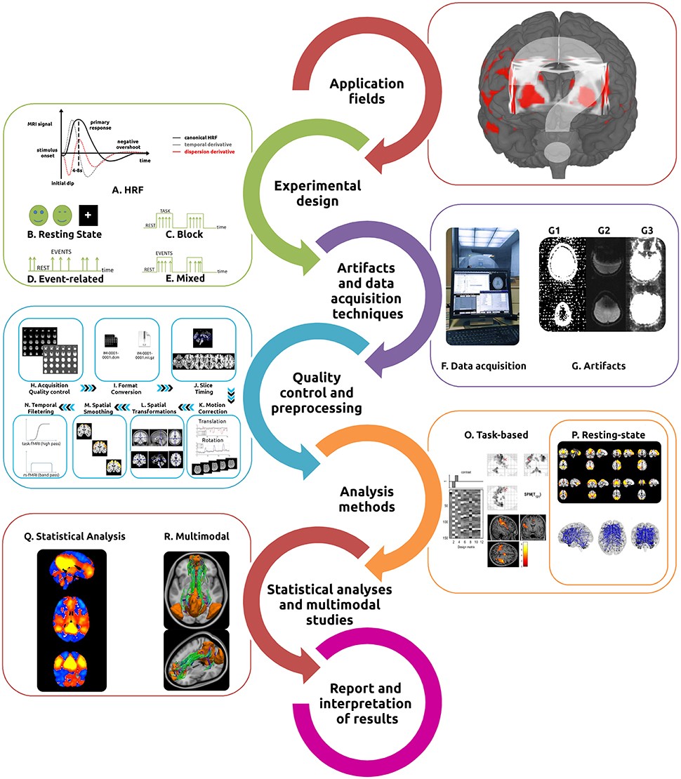
Figure 1: This illustration provides a detailed overview of the fMRI workflow. Beginning with experimental design and stimulus selection, it highlights various designs such as resting state, block, event-related, and mixed designs. Essential acquisition techniques and potential artifacts are also identified. The diagram further details the preprocessing steps involved, including acquisition quality control, format conversion, slice timing, motion correction, spatial transformations, smoothing, and temporal filtering, all leading to task-based or resting-state fMRI analysis and statistical inference.
Functional MRI studies often investigate differential neuronal responses to stimuli and activity during task performance, comparing periods of activation with baseline tasks or “rest” conditions (Bandettini et al., 1992; Blamire et al., 1992; Vallesi et al., 2015). However, spontaneous/intrinsic brain activity is also a fundamental aspect of normal brain function. Resting-state fMRI (rs-fMRI) analyses rely upon spontaneous coupled brain activity to reveal intrinsic signal fluctuations in the absence of external stimuli (Damoiseaux et al., 2006; Fox and Raichle, 2007; Schölvinck et al., 2010; van den Heuvel and Hulshoff Pol, 2010; Friston et al., 2014b).
With its increasing popularity, fMRI has shown great utility in studying the brain in health and disease. It requires knowledge of task design, imaging artifacts, complex MRI acquisition techniques, a multitude of preprocessing and analysis methods (see Tables 1–4), statistical analyses, and results interpretation.
Given the complex nature of data processing, constant methodological advances, and the increasingly broad application of fMRI, this “hitchhiker’s guide” aims to provide essential information and primary references to assist in the optimization of data quality and interpretation of results (Soares et al., 2013). We also provide an analysis of the principal software tools available for each step in the workflow, highlighting the most suitable features of each.
Applications of fMRI: A Versatile Tool for Brain Research
The versatility of fMRI has led to its application in diverse areas of cognitive neuroscience (Cabeza, 2001; Raichle, 2001; Poldrack, 2008, 2012). It has been successfully used to study systems involved with:
- Sensory-motor functions (Biswal et al., 1995; Calvo-Merino et al., 2005)
- Language (Woermann et al., 2003; Centeno et al., 2014)
- Visuospatial orientation (Formisano et al., 2002; Rao and Singh, 2015)
- Attention (Vuilleumier et al., 2001; Markett et al., 2014)
- Memory (Machulda et al., 2003; Sidhu et al., 2015)
- Affective processing (Kiehl et al., 2001; Shinkareva et al., 2014)
- Working memory (Curtis and D’Esposito, 2003; Meyer et al., 2015)
- Personality dimensions (Canli et al., 2001; Sampaio et al., 2013)
- Decision-making (Bush et al., 2002; Soares et al., 2012)
- Executive function (Just et al., 2007; Di et al., 2014)
Functional MRI has also been used as a tool in the study of topics as diverse as addiction behavior (Chase and Clark, 2010; Kober et al., 2016), neuromarketing (Ariely and Berns, 2010; Kuhn et al., 2016), and politics (Knutson et al., 2006), among others.
Clinical Applications: From Presurgical Planning to Biomarker Discovery
In clinical neuroimaging, fMRI is used for pre-surgical mapping/planning (Stippich, 2015; Lee et al., 2016), functional characterization of disease states (Matthews et al., 2006; Bullmore, 2012), studying plasticity, contributing to drug development (Wise and Preston, 2010; Duff et al., 2015), and studying genetically determined differences in function (Koten et al., 2009; Richiardi et al., 2015).
rs-fMRI has been applied to prognostic and diagnostic information (Fox and Greicius, 2010; Lang et al., 2014), treatment guidance (Rosazza and Minati, 2011; Castellanos et al., 2013), identification of functional fingerprints, discovery, and validation of biomarkers in relation to cognitive, emotional, and social processes (Fox M. D. et al., 2014; Krishnadas et al., 2014; Finn et al., 2015).
Emerging Applications: Neurofeedback and Brain-Computer Interfaces
Preliminary work shows promise for the use of real-time neurofeedback and/or brain computer interfaces (Caria et al., 2012; Weiskopf, 2012; Sulzer et al., 2013; Kadosh et al., 2016) in the treatment of disorders such as Obsessive Compulsive Disorder (Emmert et al., 2016), Depression (Young et al., 2014), and Schizophrenia (Scheinost et al., 2013; Cordes et al., 2015).
Experimental Design: Tailoring fMRI Studies to Specific Research Questions
Optimizing BOLD signal acquisition time and statistical efficiency is crucial, given the number of variables associated with each study (such as the specific nature of the research question, availability of imaging instruments, demand of data handling, and cost). Experimental designs used in fMRI are either resting state or task-based.
Resting State fMRI: Exploring Intrinsic Brain Activity
Characterization of the resting state is the most straightforward experimental design in fMRI. Subjects are not performing any explicit task (Figure 1B). Consistent and stable functional patterns, reproducible across individuals, sessions, scanners, and methods, can be identified during these acquisitions and are known as Resting State Networks (RSNs) (Fox et al., 2005; Damoiseaux et al., 2006; Long et al., 2008; Choe et al., 2015; Jovicich et al., 2016).
The specific resting conditions (eyes closed, eyes open, eyes open with fixation) and duration of the acquisition both have an important effect on the final functional signals. Scan lengths of 5–7 min provide a reasonable trade-off between time and robustness of RSNs FC (Van Dijk et al., 2010; Whitlow et al., 2011), with ~13 min scans allowing for increased reliability and greater in-depth analysis (Birn et al., 2013).
Task-Based fMRI: Evoking Brain Responses with Controlled Stimuli
When employing task-based fMRI studies, the way in which the stimuli are presented as a function of time is of upmost importance. Typical experimental designs are:
- Block designs: Present consecutive stimuli as a series of epochs, or blocks, with stimuli from one condition being presented during each epoch, followed by an epoch of stimuli from another condition, or with rest/baseline epochs (Figure 1C).
- Event-related designs: Delineate the association between brain functions and discrete events (typically randomized and of short duration between 0.5 and 8 s), separated by an inter-stimulus interval (ISI, normally ranging from 0.5 to 20 s) (Figure 1D).
- Mixed block/event-related designs: Combine stimuli in discrete blocks, providing information about both sustained and transient functional activations during task performance (Figure 1E).
The specific way with which the study conditions are modeled (model specification) also plays an important role in the signal optimization process (Price et al., 1997; Friston, 2005; Amaro and Barker, 2006; Friston et al., 2007). This includes choosing appropriate baselines and controls to allow for maximum sensitivity in the detection of brain activity related to the study target.
When designing a study involving both task-based and rs-fMRI, to avoid contamination of rs-fMRI with residual activity from previous task performance, perform the resting state acquisition before the task-based or, at the minimum, after a suitable delay (Stevens et al., 2010; Tung et al., 2013).
Software for Stimulus Programming
Several software tools can be used to implement the stated principles and present the task to the participants in the scanner (Table 2).
Table 2: This table presents a compilation of software tools commonly employed for programming and presenting stimuli in fMRI studies. It lists tools such as Presentation, E-Prime, Psychtoolbox, Cogent, and SuperLab, highlighting their utility in designing and executing experimental paradigms within the fMRI environment.
Power Analysis: Determining Adequate Sample Size
The question of “how large is enough” is a matter of debate in the neuroimaging field to determine the appropriate study sample size. Sensitivity and sensibility analyses demonstrate that sample sizes of at least 27 subjects provide adequate reliability for fMRI investigations (Thirion et al., 2007). However, a substantial number of published studies are statistically under-powered (Button et al., 2013). Use power analyses to obtain robust and meaningful findings, allowing the establishment of a sample size that will increase the confidence of detecting true effects (Ioannidis, 2008). Software tools have been developed in order to facilitate calculation of the statistical power (Mumford, 2012).
Data Acquisition Techniques and Artifacts: Minimizing Noise and Maximizing Signal
Performing effective fMRI studies requires understanding specific MRI acquisition techniques and artifacts, and how to deal with them (Figures 1F,G). Detection of the BOLD signal is the most commonly used technique in fMRI, due primarily to its ease of implementation and inherent functional contrast. Alternative detection methods exist and are based on the measurement of a combination of additional parameters including: changes in cerebral blood volume (CBV), cerebral blood flow (CBF), and cerebral metabolic rate of oxygen (CMRO2) (Davis et al., 1998).
Functional MRI data are generally collected over the entire brain through the acquisition of sequential volumes (time-points), each one composed of a set of slices. The typical sequence used for fMRI studies is echo planar imaging (EPI), which is attractive due both to its imaging speed and BOLD contrast sensitivity, but also associated with inherent artifacts and diminished image quality (Stehling et al., 1991; Poustchi-Amin et al., 2001; Schmitt et al., 2012).
Optimizing the Acquisition Phase: Parameters for Reliable Data
There is no single “gold standard” fMRI protocol due to the great variability in parameters such as the MRI hardware vendor and configuration, field strength, scanning time available, specific regions under study and subsequent analyses intended. A reasonable strategy is to start from a well-characterized “standard” protocol usually provided by the vendor, and then modify it according to the specific requirements of the study to be undertaken. Magnetic field strength is among the most defining characteristics, as increased field strengths increase sensitivity, spatial resolution, and SNR (Gore, 2003; van der Zwaag et al., 2009; Wald, 2012; Skouras et al., 2014), but at the cost of increased artifact (Triantafyllou et al., 2005).
An important trade-off in fMRI acquisition is between temporal and spatial resolution. Typical fMRI acquisitions with full brain coverage have repetition times (TRs) of 2–3 s. Due to the necessity of optimizing temporal measurements, spatial resolution is usually sacrificed. With high-field strengths and/or if full brain coverage is not mandatory for the specific study, the TR can be made as low as 1 s, or even less.
Optimizing the interval choice of echo time (TE) is critical to maximize the BOLD contrast, and is ideally equal to the apparent tissue T2*. The TE for 3 T field strength is typically around 30 ms (ranging from 25 to 40 ms) (Gorno-Tempini et al., 2002; Craddock et al., 2013; Murphy et al., 2013). An important practice is to select a flip angle equal to the Ernst angle (Ernst and Anderson, 1966) for gray matter.
Identifying and Mitigating Artifacts: Ensuring Data Integrity
The primary goal of any fMRI acquisition is to obtain the highest possible SNR and contrast-to-noise ratio (CNR) (Welvaert and Rosseel, 2013) while minimizing the impact of artifacts. The artifacts in fMRI are usually related to the pulse sequence, gradient system hardware, acquisition strategy used as well as physiological noise. Three artifacts are characteristic of the traditional EPI pulse sequence: spatial distortions, signal dropouts, and ghosting (Figure 1G).
Participant-related confounds, such as head motion (Power et al., 2012), cardiac, and respiratory “noise,” as well as vascular effects, all have a significant impact on the final fMRI results (Faro and Mohamed, 2010; Murphy et al., 2013).
The following resources can be used to minimize the impact of artifacts:
- Artifact detection Tool (ART)
- Physiological Artifact Removal Tool (PART)
- PhysIO Toolbox
- ArtRepair Software
- FMRIB’s-based Xnoisifier (FIX)
- RobustWLS Toolbox
Quality Control and Preprocessing: Refinng Data for Meaningful Analysis
Quality control and preprocessing procedures are key steps in the detection and correction of artifacts in fMRI, thus providing consistency and reliability to maps of functional activation. Although a variety of automated preprocessing pipelines have been described and implemented, there is a lack of consensus about which workflow is the most effective. Herein we provide a practical guide to the most commonly used methodologies.
Acquisition Quality Control and Data Conversion
The first quality control point comes during the acquisition phase, by assessing the images using two different contrast settings: standard anatomical (to verify the appearance of the brain, gross head motion and spiking) and background noise contrast (to verify hardware issues and important small motion) (Figure 1H). Following data acquisition, verify that all images have been imported and sorted correctly, and to ensure the same acquisition protocol has been used for all study participants. At this point, screen for obvious brain lesions and visible artifacts using general-purpose viewers, such as Osirix, MRIcro, RadiAnt, or ImageJ (Escott and Rubinstein, 2003; Rosset et al., 2004).
Due to the absence of a standard file format, convert the original scanner data from DICOM format (Mildenberger et al., 2002; Liao et al., 2008; Mustra et al., 2008) to the NIfTI format (Neuroimaging Informatics Technology Initiative), the most common file format used by fMRI preprocessing tools (Figure 1I). Several dedicated converters also are available [e.g., dcm2nii, MRIConvert and NiBabel].
Initial Stabilization, Slice-Timing, and Motion Correction
Discard the initial volumes (usually around the 10 initial seconds) of the fMRI acquisitions, whether for task-based or rs-fMRI, to remove the influence of gradient stabilization and tissue excitation.
Slice timing correction adjusts the time-course of voxel data in each slice to account for the intrinsic delay between the real and the expected slice acquisition times, by interpolating the information in each slice to match the timing of a reference slice (first or mean TR slice) (Calhoun et al., 2000; Sladky et al., 2011) (Figure 1J). For interleaved acquisitions, it is usually performed before motion correction and for sequential acquisitions thereafter.
Head motion during scanning is probably the most common and critical confound for both task and rs-fMRI studies, both of which are dependent upon precise spatial correspondence between voxels and anatomical areas over time (Friston et al., 1996; Satterthwaite et al., 2012; Maclaren et al., 2013; Zeng et al., 2014; Power et al., 2015). The most common strategy used to perform motion correction is first to realign each volume to a reference volume (mean image, first, or last volume) using a rigid body transformation (x, y, and z rotations and translations) (Jiang et al., 1995) (Figure 1K). As residual motion-induced fluctuations still are present in the data set, including the motion parameters estimated during the realignment step as “nuisance variables” (covariates of no interest), possibly also including the temporal derivatives of those variables, in the subject-level general linear model (GLM), is a different strategy that may be used (Friston et al., 1996; Johnstone et al., 2006; Power et al., 2012).
Scrubbing is based on two measures to capture the head displacements, Framewise Displacement (FD) or the brain-wide BOLD signal displacements (temporal Derivative VARiance—DVARS) derived from volume to volume measurements over all brain voxels (Power et al., 2012). After FD or DVARS calculation, a threshold is applied and outliers identified and regressed out later in the preprocessing pipeline (but before temporal filtering) from the data with a GLM where each outlier is entered as a nuisance regressor. Alternative motion correction strategies are also available, such as the use of slice derived information (Beall and Lowe, 2014), task associated motion (Artifact Detection Tool), expansion to 24–36 motion regressors (Power et al., 2014), independent component analysis de-noising (Mowinckel et al., 2012; Griffanti et al., 2014; Pruim et al., 2015), and group-level motion covariates (Van Dijk et al., 2012). Furthermore, the use of non-gray matter nuisance signals (Behzadi et al., 2007; Jo et al., 2013) and regression of global signal (Power et al., 2014) have been shown to help reducing the impact of motion.
Spatial Transformations
Performing spatial transformations to align the images from the individual’s native space with those acquired from a different modality or subject [(co-)registration] or into a common standard space (normalization) is a fundamental step of the fMRI preprocessing (Brett et al., 2002) (Figure 1L). Use either the Talairach space or the Montreal Neurological Institute (MNI) templates.
In fMRI there are two commonly used processing streams for spatial normalization. In one, a single step strategy is used to normalize directly to a standard EPI template, while the other employs a multi-step method which first aligns to the matching structural image using rigid-body or affine transformations, following which the composite image is then registered to the reference space, using either affine or non-linear transformations (Poldrack et al., 2011). Techniques for removing non-brain areas from the analysis, such as skull striping or masking, may also help to improve the normalization step (Tsang et al., 2007; Andersen et al., 2010; Fischmeister et al., 2013).
Spatial Smoothing and Filtering
The next preprocessing step normally implemented is that of spatial smoothing/filtering, a process during which data points are averaged with their neighbors, suppressing high frequency signal while enhancing low frequency ones, and results in the blurring of sharp edges (Figure 1M).
The standard spatial smoothing procedure consists of convolving the fMRI signal with a Gaussian function of a specific width [Full Width at Half Maximum (FWHM)], which determines the extent to which the data is smoothed. The choice of the proper size of the Gaussian kernel will be dependent on specific features of the study undertaken, such as type of paradigm and inference expected, as well as on the primary image resolution. The amount of smoothing always should be the minimum necessary to achieve the intended results, and a reasonable starting point is a FWHM of twice the voxel dimension. The typical smoothing values used range between 5 and 10 mm for group analyses (Beckmann and Smith, 2004; Mikl et al., 2008; Poldrack et al., 2011).
A final step in the data preprocessing pipeline is temporal filtering (Figure 1N). Perform this step to remove the effects of confounding signals with known or expected frequencies. Functional MRI time-courses often manifest low-frequency drifts which may reduce substantially the statistical power of the results. The most frequently used filters for task-based fMRI acquisitions are high-pass filters (typically ~ 0.008–0.01 Hz, 100–128 s). With rs-fMRI the standard strategy is to apply a band-pass filter (0.01–0.08 Hz). Normally associated with the filtering step, detrending methods also are used to reduce the effects of noise (Tanabe et al., 2002; Friman et al., 2004).
The use of frequency filtering (and/or spatial smoothing) may help attenuate noise and thus increase the SNR (White et al., 2001).
Software tools have been developed in order to implement quality control procedures, such as BIRN QA, NYU CBI Data Quality tool, and the CANLAB Diagnostic Tools.
Table 3: This table provides an overview of the main preprocessing steps implemented by common fMRI software tools. It includes categories such as slice timing correction, motion correction, distortion correction, spatial normalization, and smoothing, listing the specific algorithms or methods available within popular tools like AFNI, FSL, SPM, and BrainVoyager.
Analysis Methods: Unveiling Brain Activity and Connectivity
The next stage in the fMRI workflow is the selection of the most suitable method to extract the relevant functional information. There are many fMRI analysis methods and software tools for both task-based (Figure 1O) and rs-fMRI (Figure 1P). To assist with this choice, we present a table with the most commonly used software tools for the analysis of task-based and rs-fMRI data (Table 4). In the following sections we distinguish between task-based and resting-state fMRI analysis according to the prominence use of each method, nevertheless, some are suitable for both fMRI acquisitions. Other distinctions could be performed, namely between methods suitable for localization and for connectivity approaches.
Typical Task-Based Analyses Methods
The most employed method in the analysis of task-based fMRI is Statistical Parametric Mapping (SPM), which is based on the GLM (Figure 2A) (Friston et al., 1994a; Kiebel and Holmes, 2003; Poline and Brett, 2012). GLM’s popularity is based on its straightforward implementation, interpretability and computability. It incorporates most data modeling structures and provides the means for minimizing/controlling the effects of confounding factors such as motion, respiratory and cardiac and HRF derivatives (Calhoun et al., 2004; Lund et al., 2006; Bright and Murphy, 2015). The result of this process is to generate a test statistic for each voxel in the brain, which makes possible the creation of a parametric map (SPM). The process is performed separately for each subject and is commonly designated as first-level analysis. One common approach in the use of this technique is to convolve the stimulus onsets and durations with a canonical HRF, which results in quantifying an estimate of the expected BOLD signal for any condition of interest. These estimates are then defined, along with intrinsic confounding factors (e.g., motion parameters), as the independent variables of the GLM. Each voxel time-series is then set as the dependent variable. The GLM can be used very generally, ranging from the simplest subtraction method to parametric correlations with behavior, and also serves as the reference for several methods used to estimate connectivity.
Psychophysiological interaction (PPI) is used to quantify how task-specific FC between a particular brain ROI (source/seed) and the rest of the brain voxels are affected by psychophysiological variables (Figure 2B) (Friston et al., 1997; O’Reilly et al., 2012).
The structural equation model (SEM) is used to assess the effective connectivity based on an a priori model of causality (Figure 2C) (McLntosh and Gonzalez-Lima, 1994; Büchel and Friston, 1997; Kline, 2011). It starts with the definition of a set of ROIs, and then tries to determine the connection strength between those ROIs that best fit the model.
DCM allows estimation of the effective connectivity (model states) between brain regions by determining hemodynamic response (model output) as a function of specified external experimental variables (model input) (Figure 2D). One of the primary characteristics of DCM is that it allows exploration of the brain as a dynamic system, accounting for changes in populations of neurons, and is able to build non-linear models of interacting regions (Friston et al., 2003; Penny et al., 2004; Stephan et al., 2008; Friston, 2009).
Granger Causality Mapping (GCM) determines temporal precedence in neural time-series and infers causality from time-lagged correlation (Figure 2E) (Goebel et al., 2003; Friston et al., 2013; Seth et al., 2015).
Multivoxel Pattern Analysis (MVPA) uses pattern-classification algorithms (classifiers) in the attempt to delineate different mental states, as well as to correlate the patterns with specific perceptual, cognitive, or disease states (Figure 2F) (Norman et al., 2006; Mahmoudi et al., 2012; Premi et al., 2016). MVPA incorporates the signal from the distributed activity or connectivity across multiple voxels simultaneously, allowing to infer mental states from patterns of distributed neural activity.
Typical Resting State Analyses Methods
Historically, the first method applied to rs-fMRI was seed-based correlational analysis (Figure 2G) (Biswal et al., 1995). The method is based on the activity in an a priori defined ROI (the seed region) which may be a volume or a single voxel, which is compared to that in all other voxels in the brain (Lee et al., 2013).
Regional Homogeneity analysis (ReHo) (Figure 2H) uses Kendall’s coefficient of concordance to measure the synchronization between the time-series of each voxel and that of its nearest neighbors (based on a pre-defined ROI) (Zang et al., 2004). The Amplitude of Low-Frequency Fluctuations (ALFF) and more recently, the fractional ALFF (fALFF, which has reduced sensitivity to physiological noise), measures signal magnitude on a voxel by voxel basis (Figure 2I) (Zou et al., 2008).
In order to overcome the limitations of model-based analyses, exploratory data-driven methods, which require neither prior information nor a previously defined model, have been applied to fMRI. The three primary techniques are Principal Component Analysis (PCA), Independent Component Analysis (ICA), and clustering. PCA maximizes the explained variance of data and separate the relevant information from the noise (Figure 2J) (Wold et al., 1987; Viviani et al., 2005; Abdi and Williams, 2010; Smith et al., 2014). The method most frequently used for studies of rs-fMRI FC is ICA (an extension of PCA) (Figure 2K) (Jutten and Herault, 1991). This processing technique separates individual elements into their underlying components, and models the fMRI data set as a constant number of spatially or temporally independent components, which then are linearly mixed (Kiviniemi et al., 2003; Beckmann, 2012). The use of clustering methods groups data into subsets (clusters) such that parameters of the same cluster are more similar to one another than they are to those of different clusters (Figure 2L).
An increasingly prominent and powerful tool for the study of functional brain networks is graph theory. These methods model the brain as a network comprised of nodes (voxels or regions) and edges (connections between nodes, e.g., time-series correlations). This enables the establishment of functional interactions between every possible brain region, also known as the functional connectome. This whole-brain network is mathematically modeled as graph and, consequently, graph-theory metrics can be used to study the topological properties of such network (Figure 2M).
In contrast to most rs-fMRI strategies, which are based on the assumption of stationarity, dynamic functional connectivity (dFC) addresses the temporal component (fluctuations) of spontaneous BOLD signals (Figure 2N).
Figure 2: The image illustrates various analysis methods commonly used in functional MRI studies. It includes task-based analyses such as the General Linear Model (GLM), Psychophysiological Interactions (PPI), Structural Equation Modeling (SEM), Dynamic Causal Modelling (DCM), Granger Causality Mapping (GCM), and Multi-voxel Pattern Analysis (MVPA). Additionally, it presents methods for analyzing resting-state fMRI data, such as seed-based correlations, Regional Homogeneity (ReHo), Amplitude of Low Frequency Fluctuations (ALFF), Principal Component Analysis (PCA), Independent Component Analysis (ICA), Clustering, Graph Theory, and dynamic Functional Connectivity (dFC).
Table 4: This table presents a detailed list of the main analysis methods implemented by common fMRI tools. It includes various tools and their capabilities in preprocessing, statistical analysis, and advanced modeling techniques suitable for both task-based and resting-state fMRI data.
Statistical Analyses: Drawing Meaningful Conclusions from fMRI Data
In a single fMRI experiment, images made up of roughly 100,000 voxels are acquired from hundreds to thousands of times, resulting in a massive data set which has a complex spatial and temporal structure.
Group-Level Analyses
In order to make inferences at the group-level (i.e., second-level), the analyses of fMRI data most widely used are performed within the GLM framework. Hypothesis testing in the GLM framework include a set of parametric approaches, comprising the familiar T-Tests (independent and paired), Multiple Regression and ANalysis Of VAriance (ANOVA) (Friston et al., 2007). Commonly, the research question leads to more complex experimental designs which involve both within-subjects (e.g., condition A vs. B) and between-subjects (e.g., control vs. experimental group) factors. Parametric tests are popular due to their simplicity and ease of application. However, these tests make some strong assumptions that are minimally met, or not met at all, in fMRI data sets (e.g., assumption of normality). As a result, it is often more appropriate to use non-parametric tests. Such tests estimate the null distribution from the data itself. The most common non-parametric tests used in fMRI analysis are permutation (randomization) tests. Tools that implement such tests include randomize from FSL and SnPM.
Statistical Significance
As in all standard statistical inference, the evaluation of fMRI data requires establishing a criterion for statistical significance. Early fMRI studies commonly used an uncorrected p–