Colocalization analysis in biological microscopy is pivotal for understanding molecular interactions within cells, and CONDUCT.EDU.VN offers an invaluable resource. This practical guide details evaluating colocalization, enhanced by cutting-edge techniques and optimized for search engines, ensuring researchers and students can effectively quantify molecular co-occurrence and associations, boosting research validity and replicability. Explore concepts like image analysis and fluorescence microscopy to deepen your understanding.
1. Understanding Colocalization in Biological Microscopy
Fluorescence microscopy stands as an essential method for exploring the roles of proteins and other molecules within cells. A fundamental part of this technique involves determining if two or more molecules are found in the same locations or structures within a cell, an idea known as “colocalization.” By understanding colocalization, scientists can deduce the functions of molecules, such as finding out if a protein connects with a specific part of a cell or a molecular complex.
1.1. Defining Colocalization
Colocalization, in the context of biological microscopy, involves assessing the distribution of signals in fluorescence microscopy images to ascertain whether two probes, typically fluorescently labeled molecules, co-distribute or associate with one another. This means analyzing if the fluorescent signals from these molecules overlap in specific cellular locations.
1.2. Limitations of Visual Assessment
While visual inspection of merged images is a common first step, it can be subjective and misleading due to variations in probe intensities and the potential for misinterpretation of overlapping signals. Quantitative methods offer a more robust and objective assessment of colocalization.
1.3. Relevance to Molecular Interactions
It is critical to note that while colocalization can suggest associations between molecules, it does not confirm direct molecular interactions. The resolution limits of light microscopy prevent the identification of physical apposition of two molecules based solely on their distribution in fluorescence images.
1.4. Applications of Colocalization Analysis
Colocalization analysis is suitable for determining whether two molecules are found within the same structures or compartments, such as endosomes, mitochondria, or specific plasma membrane domains. It can also reveal if proteins associate with subnuclear structures.
2. Visual Methods for Evaluating Colocalization
Visual methods for evaluating colocalization involve examining fluorescence microscope images to subjectively assess the co-occurrence of two or more fluorescently labeled molecules. These methods primarily rely on the visual appearance of structures whose color suggests the combined presence of both probes.
2.1. Superposition of Fluorescence Images
The most common method is the superposition of images, where images of different probes are merged to visualize their spatial relationships. This method can reveal if two probes co-occur in the same structures, indicated by a combined color.
For example, in the case of fluorescein (green) and rhodamine (red) labeled molecules, colocalization is indicated by a yellow color, reflecting the combined contributions of both probes in the same location.
2.2. Limitations of Superposition
While superposition provides a spatial sense of colocalization, it has limitations. The intermediate color that suggests colocalization is obtained only if the intensities of the two probes are similar. Small changes in the relative intensity of two probes can completely alter the combined color of structures, affecting the perception of probe colocalization.
2.3. Side-by-Side Comparison
To overcome the limitations of superposition, a reliable method for visually comparing the relative distribution of two probes is a side-by-side comparison of the individual images, which allows for a direct assessment of their spatial relationships.
2.4. Scatterplots
Scatterplots offer additional insights into colocalization studies by graphically representing the intensity of one color against the intensity of the second color for each pixel. This representation is similar to the output provided for flow cytometry data.
When proportional codistribution is present, the points of the scatterplot cluster around a straight line, whose slope reflects the ratio of the fluorescence of the two probes. In contrast, a lack of colocalization is reflected by the distribution of points into separate groups, each showing varying signal levels of one probe with little or no signal from the other probe.
2.5. Identifying Distinct Compartments
Scatterplots can identify populations of distinct compartments with different ratios of the two probes, allowing for the identification of multiple compartments with distinct molecular compositions.
2.6. Qualitative Indication of Colocalization
While visual techniques provide a spatial sense of colocalization and can identify distinct populations of compartments, they are not helpful for comparing the degree of colocalization in different experimental conditions or for determining whether the amount of colocalization exceeds random coincidence.
3. Quantifying Colocalization
To objectively and reproducibly assess the extent of colocalization, quantitative methods are essential. These methods provide numerical values that allow for statistical comparisons and a more precise understanding of molecular co-occurrence.
3.1. Pearson’s Correlation Coefficient (PCC)
Pearson’s correlation coefficient (PCC) is a widely used statistic for quantifying colocalization. It measures the pixel-by-pixel covariance in the signal levels of two images.
PCC values range from +1 for two images whose fluorescence intensities are perfectly, linearly related, to -1 for two images whose fluorescence intensities are perfectly, but inversely, related to one another. Values near zero reflect distributions of probes that are uncorrelated with one another.
3.2. Advantages of PCC
The primary advantage of PCC is its simplicity. It measures the degree to which the variability in red and green pixel intensities can be explained with a simple, linear relationship between the two. Because it subtracts the mean intensity from each pixel’s intensity value, PCC is independent of signal levels and signal offset (background).
3.3. Limitations of PCC
PCC is sensitive to both signal co-occurrence and signal correlation. If the distribution of two probes is not expected to overlap proportionally, PCC can provide a poor measure of colocalization.
PCC values can be depressed if measured over a field of cells with heterogeneous expression or uptake of the target molecules.
3.4. Region of Interest (ROI)
PCC should generally be measured for individual cells by hand-drawing a “region of interest” (ROI) over the image.
3.5. Influence of Extracellular Regions
Unlabeled extracellular regions can artificially inflate PCC values if included in the region of measurement. It is critical to carefully outline the region in which two probes may potentially distribute.
3.6. Excluding Irrelevant Pixels
Regions within the cell that exclude the structures of interest may also inflate PCC measurements. An alternative approach for excluding irrelevant pixels is to restrict analysis to pixels whose intensity falls above a threshold value.
3.7. Biological Conditions for PCC
To productively use PCC to measure colocalization, it is important that investigators understand exactly what PCC measures. To the degree that the biology of the system is such that can be modeled by a linear relationship in the levels of two probes, PCC is an appropriate measure of association.
3.8. Cases Where PCC Measurements are Ambiguous
In cases where probes co-occur in different proportions in different compartments of the cell, PCC values will be depressed if measured in a population of heterogeneous intracellular compartments.
Even if two probes co-occur on the same cellular structures, there may be no reason that they should co-occur in fixed proportion to one another. In such cases, PCC can provide a poor measure of colocalization.
3.9. Restriction of Measurements to Pixels That Contain Both Fluorophores
Limiting measurements to pixels that contain both probes changes the parameter that is measured by PCC. If one is interested in evaluating the distribution of a probe, the regions from which the probe is excluded are as meaningful as those in which the probe is found.
4. Manders’ Overlap Coefficient (MOC)
Manders’ Overlap Coefficient (MOC) is an alternative metric developed in response to the perceived difficulty of interpreting negative PCC values. MOC is calculated using the formula:
MOC = Σ(Ri × Gi) / √(ΣRi^2 × ΣGi^2)
4.1. Implementation of MOC
MOC is implemented in image analysis software packages, such as Colocalizer Pro, Image-Pro, Imaris, and Volocity, and can be implemented in ImageJ via the JACoP plugin.
4.2. Consequences of Eliminating the Subtraction of Mean Signals
Eliminating the subtraction of mean signals from the equation prevents negative MOC values but has other consequences. MOC is almost independent of signal proportionality and is primarily sensitive to co-occurrence, the fraction of pixels with positive values for both channels, regardless of signal levels.
4.3. MOC as an Indicator of Colocalization
The insensitivity of MOC to signal proportionality might suggest MOC as a better indicator of colocalization than PCC for some analyses. However, MOC only indirectly and somewhat unpredictably measures co-occurrence.
5. Fractional Overlap
Fractional overlap is measured via Manders’ Colocalization Coefficients (MCC), which are widely used in biological microscopy. These coefficients provide measures of the fraction of total probe fluorescence that colocalizes with the fluorescence of a second probe.
5.1. Manders’ Colocalization Coefficients (MCC)
For two probes, denoted as R and G, two different MCC values are derived: M1, the fraction of R in compartments containing G, and M2, the fraction of G in compartments containing R. These coefficients are calculated as follows:
M1 = ΣRi,colocal / ΣRi
where Ri,colocal = Ri if Gi > 0 and Ri,colocal = 0 if Gi = 0
M2 = ΣGi,colocal / ΣGi
where Gi,colocal = Gi if Ri > 0 and Gi,colocal = 0 if Ri = 0
5.2. Measures of the Fraction of Total Probe Fluorescence
By providing measures of the fraction of total probe fluorescence that colocalizes with the fluorescence of a second probe, MCCs provide an intuitive and direct metric of the quantity of interest for most biological colocalization studies.
5.3. Independent of Signal Proportionality
Unlike PCC, MCC strictly measures co-occurrence independent of signal proportionality.
5.4. Eliminating the Component of Pixel Intensity
While simple in principle, measuring MCC is complicated by the fact that the input values used to measure MCC can almost never be taken directly from the original images. Since MCC depends utterly upon the ability to distinguish pixels with signal derived from a labeled structure in the focal plane from pixels whose signal results strictly from background sources, a necessary preliminary step is to eliminate the component of pixel intensity derived from background.
5.5. Methods for Eliminating Background
The most obvious method for eliminating background is to subtract a global threshold value from the pixel intensities of the image.
5.6. Challenges in Estimating the Appropriate Threshold Value
For many images, estimating the appropriate threshold value representing background is challenging. For images in which much of the fluorescence occurs in structures whose intensity is close to that of the background, MCC is very sensitive to the value chosen for the threshold.
5.7. Costes Automatic Thresholding Method
Costes et al. developed a unique approach for automatically identifying the threshold value to be used to identify background based on an analysis that determines the range of pixel values for which a positive PCC is obtained.
5.8. Method for Estimating Thresholds
The Costes method for estimating thresholds is a robust and reproducible method that can be easily automated, both speeding processing and eliminating user bias. The method has been implemented in the Imaris, Slidebook, and Volocity software and in ImageJ plugins (JACoP, WCIF).
5.9. When the Costes Procedure Can Fail
Under some circumstances, the Costes procedure can fail to identify a useful threshold. For example, previous studies have shown that Costes thresholding struggles with images that have very high labeling density or large differences in the number of structures labeled with each probe.
5.10. Sensitivity to the Estimate of Background
MCC is very sensitive to the estimate of background, indicating the importance of an automatic, or at least nonsubjective, reproducible method for determining background.
5.11. Spatial Variation in Background
The Costes approach fails to address a more general problem for thresholding images: background levels vary spatially in many cases so that no one background value is appropriate for the entire image.
5.12. Local Background
For studies of dispersed objects, an effective measure of local background can be derived from the median intensity in a relatively large region surrounding each pixel in the image.
5.13. Image Spatially Filtered
In this approach, the image is spatially filtered to remove pixel noise and a background image is constructed in which the value of each pixel in the original image is replaced with the median intensity in the region surrounding the pixel. This background image is then subtracted pixel-by-pixel from the filtered image to obtain a background-subtracted quotient image.
5.14. Applying the Median Subtraction Method
The size of the region is critical; it must be large enough to predominantly measure the region surrounding objects but small enough to reflect spatial variation.
6. Comparison of Pearson’s Correlation Coefficient and Manders’ Colocalization Coefficient
Pearson’s Correlation Coefficient (PCC) and Manders’ Colocalization Coefficient (MCC) represent the two major metrics of colocalization used in biomedical research. Strictly speaking, neither is superior to the other; both have strengths and weaknesses that, depending on the situation, make one or the other the preferred metric.
6.1. Advantages of MCC
The most obvious advantage of MCC is that it is a more intuitive measure of colocalization than PCC. MCC is also more useful for data that are poorly suited to the simple, linear model that underlies PCC.
6.2. Probe Distributions
MCC provides two components: the fraction of A with B and the fraction of B with A. This is important when the probes distribute to different kinds of compartments, as for example, in the case in which all of A is found in compartments containing B, but B is also found in additional compartments lacking A.
6.3. Three-Dimensional Analysis of Colocalization
MCC analysis is also more appropriate for three-dimensional analysis of colocalization, which is required for studies in which probe colocalization varies spatially in a cell.
6.4. Quantification of an Overall PCC for a Three-Dimensional Volume
Quantification of an overall PCC for a three-dimensional volume of the cell requires delineation of the region-of-interest for each focal plane from the volume and combination of all of the identified voxels into a single array from which PCC is calculated. Since MCCs are not influenced by areas from which both probes are excluded, MCC does not require this painful delineation of the region-of-interest.
6.5. Application to Three-Dimensional Analyses
MCC analysis is also much easier to extend to three-dimensional analyses (in which case it is sometimes called an “object-based” analysis).
6.6. Measuring PCC in a Projected Image of the Volume
A simpler alternative to three-dimensional analysis that frequently yields comparable results is to measure PCC in a projected image of the volume.
6.7. When Projection Yields Comparable Results
This approach is best limited to cells with limited depth and label density such that structures do not overlap when projected into a single image.
6.8. Generating Spurious Estimates of Overlap
MCC analysis is less forgiving of overlap occurring in the projection process and should seldom be applied to projected data, where it is likely to generate spuriously high estimates of overlap.
6.9. Main Drawback of MCC
The major drawback of MCC is that it is complicated by the need to be able to reliably identify background levels in an image and thereby identify labeled structures.
6.10. Choice of a Thresholding Method
Given the subjectivity, it is important to avoid bias by consistently applying the same thresholding technique to all experimental samples. For some images, effective thresholding can be accomplished by relatively standard methods. However, many images obtained in biological microscopy are challenging for standard thresholding techniques and may require more elaborate methods of image segmentation.
6.11. PCC as the Preferred Method
For images where background correction is challenging, PCC analysis may still be the preferred method, as it requires no image preprocessing of any kind.
7. Significance Testing in Colocalization Studies
Significance testing in colocalization studies is often overlooked but crucial for validating results. It helps determine if the observed colocalization is statistically significant or merely due to random chance. Two primary forms of significance testing are used: comparing colocalization between experimental groups and assessing the significance of colocalization within a single group.
7.1. Noise
Before discussing significance testing, understanding the concept of noise is essential. Noise refers to the variability in a measurement, distinct from background, which is the offset in an image. Noise can affect PCC by causing it to decline, and it complicates thresholding for MCC. Minimizing noise during image collection is crucial for accurate colocalization analysis.
7.2. Significance in Differences Between Experimental Groups
Statistical tests, like Student’s t-tests, can be used to test the significance of differences in PCCs and MCCs between experimental groups. This approach is valid as long as confounding variables, such as differences in signal level, noise, or the accuracy of background estimation, are consistent between groups.
7.3. Estimating Significance for a Single Group
Estimating the significance of a colocalization measurement made for a single group is more challenging. It involves comparing the measured value to a “null” model, representing the measurement expected from random data.
7.4. Statistical Significance of a Measured PCC Value
The statistical significance of a measured PCC value can be derived directly from the data, based on the deviations of individual values from the best-fit regression line and the number of measurements. However, with large sample sizes in image analysis, even subtle and biologically meaningless correlations can result in statistically significant PCC values.
7.5. Optical Artifacts
Correlations can result from optical artifacts like gradients in the field of illumination or lack of flat-field correction in the microscope objective.
7.6. Spatial Autocorrelation
Significance testing of correlation coefficients is confounded by spatial autocorrelation, where the value of one pixel is likely to be similar to that of its neighboring pixels. Autocorrelation can result in statistically significant correlations even for variables with no real association, leading to overly low P values.
7.7. Alternative Approach
An alternative approach is to compare the mean of measured values to the mean obtained from pairs of images that are out of registration with one another.
7.8. Randomization Approach
The most accurate method for estimating the significance of a colocalization measurement is based on comparison with a large number of measurements taken in comparable samples in which the distributions of the two probes are unrelated. However, since such samples seldom exist, a practical alternative is a randomization approach in which the random probability distribution is generated from measurements of images in which one channel is scrambled or translated.
7.9. Scrambling Approach
In the scrambling approach, the random probability distribution is derived from repeated measurements of colocalization between the image of one channel and a version of the second channel in which the pixels or blocks of pixels are randomly rearranged.
7.10. Frame-Translation Approach
In the “frame-translation” approach, the random probability distribution is derived from a number of measurements obtained after translating the image of one channel relative to the other.
7.11. Eliminating Spatial Autocorrelation
Unfortunately, the scrambling approach is complicated by autocorrelation. Rearranging the individual pixels of one channel eliminates the spatial autocorrelation of that channel.
7.12. Scrambled Image Using Blocks of Pixels
The accuracy of the probability distribution can be improved by generating the scrambled image using blocks of pixels rather than individual pixels.
7.13. Pixel Block Scrambling Approach
The pixel block scrambling approach for estimating the random probability of a colocalization measurement has been implemented in the Slidebook image analysis software package and the JACoP and WCIF ImageJ plugins, which include the capability to adjust the block size used in randomization.
7.14. Avoiding Spatial Autocorrelation
The problem of spatial autocorrelation can be avoided using a frame translation approach, in which the random probability distribution is generated from measurements of colocalization obtained after shifting one image relative to the other.
7.15. Wrap-Around Technique
One way to increase the number of random measurements in a frame-translation method is to apply a “wrap-around” technique, in which translated regions that depart the region of interaction are populated with pixels from the opposite side of the region.
7.16. Limitations in Practical Application
Both of the randomization approaches are complicated by the need to identify the region of potential interaction between the two probes.
7.17. Accurately Estimating Randomized Data
Failure to appreciate these factors will generally lead to systematic overestimation of the significance of colocalization measurements.
7.18. Solving Significance Testing
The problem of significance testing of colocalization data is one with no simple answer at this point.
8. An Outline of a Colocalization Analysis Workflow
To make sense of these considerations, a structured workflow is essential for conducting colocalization analysis effectively. This section outlines the key steps involved in the colocalization analysis process.
8.1. Identifying the Nature of Colocalization
The initial step in colocalization analysis is to identify the nature of the colocalization question.
8.2. Designing and Conducting Image Collection
The next step in colocalization analysis is to design and conduct image collection.
8.3. Determining Quantification
The investigator needs to determine whether quantification is necessary.
8.4. Choosing Between PCC and MCC
If quantification is desired, the choice for most studies is between some form of PCC and MCC.
8.5. Evaluating the Linearity
Data should first be evaluated for linearity by plotting the values of a few representative cells in scatterplots.
8.6. Measuring Probe Colocalization
If the data indicate a simple linear relationship, one should then randomly identify cells to be quantified and outline the relevant ROI for each.
8.7. Defining the Region of Interest
Since MCCs are not influenced by areas from which both probes are excluded, MCC does not require this painful delineation of the region-of-interest.
8.8. Defining the Estimated Level of Background
The major drawback of MCC is that measured values are very sensitive to the estimated level of background, the threshold value used to distinguish labeled structures from unlabeled background.
8.9. Software to Evaluate Effects of Parameter Adjustments
Software that provides the ability to visually evaluate the effects of parameter adjustments is preferable to software that simply spits out a final numerical value.
9. Final Thoughts
Colocalization analysis in fluorescence microscopy demands a careful approach, emphasizing thoughtful application of both visual and quantitative methods. By understanding the strengths and limitations of different techniques like PCC and MCC, and by rigorously validating image processing steps, researchers can derive meaningful and reliable insights into molecular interactions.
The pursuit of knowledge in biological microscopy should be driven by curiosity and guided by meticulous methodology. For further guidance, resources, and support in navigating the nuances of colocalization analysis, visit CONDUCT.EDU.VN. Your commitment to excellence in research is paramount, and CONDUCT.EDU.VN is here to assist you every step of the way.
For support or inquiries, please contact us:
Address: 100 Ethics Plaza, Guideline City, CA 90210, United States
WhatsApp: +1 (707) 555-1234
Website: CONDUCT.EDU.VN
10. Frequently Asked Questions (FAQs)
-
What is colocalization in biological microscopy?
- Colocalization refers to the co-occurrence of two or more molecules in the same location within a cell, as observed using fluorescence microscopy. It suggests potential interactions or shared functions between these molecules.
-
Why is colocalization analysis important?
- Colocalization analysis helps researchers understand molecular interactions, cellular processes, and the functional relationships between different molecules within cells.
-
What are the key methods for assessing colocalization?
- Key methods include visual assessment (superposition of images), Pearson’s Correlation Coefficient (PCC), and Manders’ Colocalization Coefficients (MCC).
-
What is Pearson’s Correlation Coefficient (PCC)?
- PCC is a statistical measure that quantifies the linear relationship between the intensities of two probes. It ranges from -1 to +1, where +1 indicates perfect positive correlation, -1 perfect negative correlation, and 0 no correlation.
-
What are Manders’ Colocalization Coefficients (MCC)?
- MCC measures the fraction of one probe that colocalizes with another. It provides two values: the fraction of probe A that overlaps with probe B, and the fraction of probe B that overlaps with probe A.
-
How do I choose between PCC and MCC?
- Choose PCC if you expect a linear relationship between the probes and want to assess overall correlation. Choose MCC if you want to quantify the degree of overlap independent of signal proportionality.
-
What is the Costes method for thresholding?
- The Costes method is an automated approach for determining the threshold value to distinguish signal from background. It identifies the range of pixel values for which a positive PCC is obtained.
-
What is spatial autocorrelation, and why is it important?
- Spatial autocorrelation refers to the tendency of neighboring pixels to have similar values. It can confound statistical significance testing by inflating P values.
-
How can I account for spatial autocorrelation in colocalization analysis?
- You can use randomization approaches like pixel scrambling or frame translation to generate random probability distributions that account for spatial autocorrelation.
-
Where can I find more resources on colocalization analysis?
- You can find additional resources, guidelines, and support at conduct.edu.vn, including detailed articles and practical tips for conducting colocalization analysis.