A Practical Guide to Immunoassay Method Validation

Immunoassays, such as Enzyme-Linked Immunosorbent Assays (ELISAs), are crucial for quantifying low-abundance biomarkers in clinical medicine, research, and drug development, particularly in areas like Alzheimer’s disease. However, the variability in ELISA method quality necessitates stringent assay performance control. Method validation provides objective evidence that a method meets the requirements for its intended use. While extensive literature exists on validation parameters, detailed guidance on performing experiments is lacking. This guide provides step-by-step standard operating procedures (SOPs) and a validation report template for comprehensive immunoassay validation, applicable across various analytical technologies and suitable for multicenter evaluations.

Introduction

Biochemical markers are essential in clinical decision-making, including diagnosis, treatment monitoring, and prognosis prediction. In Alzheimer’s disease (AD) research, cerebrospinal fluid (CSF) biomarkers such as β-amyloid 42 (Aβ42), total tau (T-tau), and phosphorylated tau (P-tau) exhibit high diagnostic accuracy, even in early stages. These biomarkers are utilized in clinical trials as diagnostic and theragnostic markers and in clinical studies of disease pathogenesis. Immunoassays, particularly ELISA, are vital for measuring these low-abundance proteins. Reliable and reproducible results require robust assay performance control and standardized reporting.

Method validation confirms that a method reliably produces results for its intended use. Specifying the method’s intended use is crucial before validation experiments. This paper focuses on validating methods for determining analyte concentrations in biofluids, such as using the outcome as a diagnostic marker. In this case, evidence of a disease-dependent change in analyte concentration is required. The magnitude of this change influences the required method precision, analytical sensitivity, and specificity.

While much has been published on method validation, a consensus protocol is lacking due to varying requirements across analytical technologies and limited international dissemination of national initiatives. For example, carryover is relevant in chromatography but not in ELISA. This work presents straightforward SOPs for validating methods that determine analyte concentrations in biofluids, designed for ease of use without extensive prior training.

This guide is the primary deliverable of the “Development of assay qualification protocols” sub-task within the BIOMARKAPD project, supported by the European Union Joint Programme – Neurodegenerative Disease Research. The BIOMARKAPD project aims to standardize biomarker measurements for AD and Parkinson’s disease (PD), covering pre-analytical and analytical procedures, assay validation, and development of reference measurement procedures (RMP) and certified reference materials (CRM) for harmonization. The project involved drafting, reviewing, and revising SOPs, followed by evaluation in multicenter studies. End-user feedback and subsequent reviews led to final, consensus SOPs that form the basis of this report.

Full vs. Partial Validation

This guide includes SOPs for 10 validation parameters. Full validation, encompassing all parameters, is recommended for in-house methods. Partial validation of commercial assays should include all parameters except robustness, typically addressed by the manufacturer. Limited partial validations may be appropriate in specific scenarios. For instance, when transferring a validated in vitro diagnostic (IVD) method to a new lab, revalidating precision and quantification limits may suffice, as these are sensitive to changes, whereas dilution linearity and recovery are less likely to be affected.

Collaboration with the client or sponsor is essential to define the validation scope. ISO 15189, designed for clinical laboratories, offers limited guidance, stating only that “The validations shall be as extensive as are necessary to meet the needs in the given application or field of application.”

Validation Report

Laboratories seeking accreditation to international standards face stringent documentation requirements. ISO 15189 mandates recording results and procedures used for validation. A validation report template, adapted from a Swedish handbook and available in Data Sheet S1 in Supplementary Material, facilitates this process. Table 1 provides a brief description of the 10 validation parameters. Data Sheet S2 in Supplementary Material aids in extracting information from measurement data.

Robustness

Robustness, or ruggedness, refers to a method’s ability to withstand minor variations in parameters. For commercial assays, manufacturers should provide robustness assessment data. For in-house methods, robustness should be assessed during method development, and results should be incorporated into the assay protocol before further validation. Validations are tied to specific protocols, so protocol changes may necessitate revalidation.

Procedure

1. Identify critical parameters such as incubation times and temperatures.
2. Systematically alter these parameters, one at a time, while analyzing the same sample set.
3. If measured concentrations remain unaffected, adjust the protocol to include appropriate intervals, e.g., 30 ± 3 min or 23 ± 5°C.
4. If changes systematically alter concentrations, reduce the change magnitude until no dependence is observed. Incorporate these findings into the protocol.

Note: Software like MODDE (Umetrics) or published methods can reduce the number of experiments needed when many critical steps are identified.

Precision

Precision indicates the closeness of agreement between independent test results under specified conditions. There are three types of precision: repeatability (r), intermediate precision (Rw), and reproducibility (R). Repeatability measures variability when factors like laboratory, technician, day, instrument, and reagent lot are kept constant and the time between measurements is minimal. Reproducibility involves varying all factors and conducting measurements over several days. Intermediate precision allows all factors except the laboratory to vary. Report the varied factors in the validation report. Repeatability is also known as within-run or within-day precision, while intermediate precision is known as between-run or between-day repeatability.

Imprecision, the inverse of precision, is commonly reported using standard deviation (SD) and coefficient of variation (%CV) for different levels of the measurand, e.g., %CVRw. Analysis of variance (ANOVA) is used to estimate imprecision, and an Excel file (Data Sheet S3 in Supplementary Material) uses formulas from ISO 5725-2 for calculations.

Procedure

1. Collect samples with known high and low measurand concentrations. Pool samples if necessary.
2. Make 25 aliquots of each sample and store them at −80°C pending analysis.
3. Measure five replicates of each sample on days 1–5 (not necessarily consecutive).
4. Enter data, with separate days on different rows, into the Excel file Data Sheet S3 in Supplementary Material, which calculates the mean, SD, and %CV for repeatability and intermediate precision.

Five samples covering a wide measuring range are generally recommended. However, two carefully chosen levels, one above and one below the decision limit, may suffice. Obtaining samples covering a wide range may be challenging, especially when patient and control levels are similar or undefined. Prepare more aliquots than needed for precision measurements for use as internal quality control samples once the method is implemented.

Alternative experimental schemes are possible, such as 12 replicates on one day and three replicates on four different days, or, as recommended by the Clinical and Laboratory Standards Institute, two separate runs on 20 days (40 runs total). The latter allows for exploring more factors but is impractical and expensive for commercial ELISA kits with limited calibrator curves per package.

Trueness

Trueness is the closeness of agreement between the average value from a large series of test results and an accepted reference value. Ideally, the reference value comes from a CRM or materials traceable to a CRM. Bias (b) quantifies trueness, representing the systematic difference between the test result and the accepted reference value.

Procedure

1. If a CRM exists, calculate the bias (bCRM) using formula (1), where the measured mean value (X¯) is calculated from five replicates, and xref is the assigned reference value.
2. If an external quality control (QC) program exists but no CRM, calculate the bias (bQC) as the mean deviation from assigned QC values using formula (2). Note that bias may be concentration-dependent, so bQC should be calculated using a longitudinal QC sample.

Formulas:

bCRM=X-¯Xref

bQC=∑i=1nXi−XQCin

where n is the number of measurements, xi is the value measured in the laboratory, and xQCi is the value from the ith sample in the QC program.

Determined bias can be used to compensate for measured concentrations, resulting in a method without systematic effects. For constant bias over the measurement interval, subtract the bias from the measured value. If the bias is proportional to the measured concentration, correct by multiplying by a factor determined from bias evaluations at different concentrations. Alternatively, assign new values to the calibrators to compensate for bias. The total bias comprises components from the method and the laboratory. Manufacturers should calibrate their methods against materials traceable to a CRM; thus, the total bias should ideally equal the laboratory bias.

Uncertainty

Intermediate precision indicates the dispersion of results within a laboratory, regardless of the true value of the measurand. In the absence of a CRM, measurements provide relative concentrations. A CRM is needed if different methods are used to quantify the same analyte and a universal cutoff value is required. This allows kit manufacturers to calibrate their methods and minimize bias. Absolute concentrations can then be calculated, but the uncertainty must include both the method uncertainty and the uncertainty of the assigned CRM value.

Procedure

1. If a CRM exists, calculate the combined uncertainty (uc) from the standard uncertainty of the precision (uprecision) and the CRM (uCRM) using formula (3). Both uprecision and uCRM must be SDs. This calculation assumes that the bias has been adjusted, as outlined in the trueness section. Results from precision measurements can be used to estimate uncertainty, e.g., uprecision = sRW.
2. Calculate the expanded uncertainty (U) using formula (4). The coverage factor (k) is typically set to 2 for a confidence interval of approximately 95%. The coverage factor depends on the degrees of freedom.

Formulas

uc=uprecision2+uCRM2

U=k⋅uc

Limits of Quantification

The working range of a method is defined by the lower and upper limits of quantification (LLOQ and ULOQ, respectively). The LLOQ can be defined based on instrument signals or calculated concentrations.

Procedure (Signal-Based)

1. Run 16 blank samples (immunodepleted matrix or sample diluent).
2. Calculate the mean and SD of the signal.
3. Determine the concentration based on a signal of 10 SDs above the mean of the blank. Note: This only provides the LLOQ, not the ULOQ.

To determine the concentration based on a signal, use the inverse of the calibration function. The four and five-parameter logistic models are common in immunochemical calibrations.

The four-parameter logistic function and its inverse are:

Signal= A − D 1 + Concentration CB + D ⇔Concentration= C A − D Signal − D −1 1 B

For the five-parameter logistic model, the corresponding functions are:

Signal= A − D 1 + Concentration CBE + D ⇔Concentration= C A − D Signal − D −1 1 E −1 1 B

The parameters A–E are available from data acquisition and analysis software.

Based on concentrations, the LLOQ and ULOQ can be defined as the endpoints of an interval in which the %CV is below a specific level, with a potentially higher %CV at the endpoints.

Procedure (Concentration-Based)

1. Analyze, in duplicate, samples with very low and very high concentrations of the measurand.
2. Calculate the average concentration and %CVs for the samples.
3. Create a scatter plot of %CV as a function of concentration.
4. Determine the LLOQ by identifying the lowest mean level above which the %CV is < 20% for most samples.
5. Determine the ULOQ by identifying the highest mean level below which the %CV is < 20% for most samples.

Dilution Linearity

Dilution linearity demonstrates that a sample with a spiked concentration above the ULOQ can be diluted to a concentration within the working range while still providing a reliable result. It determines the extent to which the dose-response of the analyte is linear in a specific diluent within the standard curve range. Dilution of samples should not affect accuracy and precision. This also investigates the presence of a hook effect, i.e., signal suppression at concentrations above the ULOQ.

Procedure

1. Spike three undiluted samples with calibrator stock solution to the highest possible concentration. Ideally, spike samples with 100- to 1000-fold the concentration at ULOQ using the calibrator stock solution. Biological samples can also be diluted less than the prescribed concentration if an assay allows.
2. Serially dilute the spiked samples using sample diluent in small vials until the theoretical concentration is below the LLOQ. Perform dilutions in vials, not directly in ELISA plate wells.
3. Analyze the serial dilutions in duplicate and compensate for the dilution factor.
4. Calculate the mean concentration for dilutions within the LLOQ and ULOQ range. Also, calculate the %Recovery for the calculated concentration at each dilution. The calculated concentration for a dilution within the LLOQ and ULOQ range should meet the precision acceptance criteria defined in the “SOP for fit-for-purpose,” as should the calculated SD. Plot the signal against the dilution factor to investigate signal suppression at concentrations far above the measurand’s ULOQ (“hook effect”).

Dilution linearity differs from linearity of quantitative measurement procedures as defined by CLSI, which pertains to the calibration curve’s linearity.

Parallelism

Parallelism and dilution linearity share conceptual similarities. In dilution linearity, samples are spiked with the analyte to such high concentrations that the sample matrix effect is negligible after dilution. In contrast, parallelism involves using only samples with high endogenous analyte concentrations, but below the ULOQ, without spiking. The goal is to verify that the binding characteristics of the endogenous analyte to antibodies are the same as for the calibrator.

Procedure

1. Identify four samples with high endogenous concentrations of the measurand, below the ULOQ.
2. Make at least three two-fold serial dilutions using sample diluent in reaction vials until the calculated concentration is below the LLOQ. Adjust the dilution factor to obtain concentrations evenly spread across the standard curve. For example, use a dilution factor of 10 if a standard curve includes values between 0.1 and 200 pg/ml.
3. Analyze the neat samples and serial dilutions in duplicate within the same run, and compensate for the dilution factor.
4. For each sample, calculate the %CV using results from the neat sample and dilutions.

Acceptance criteria for %CV to demonstrate parallelism vary. Some suggest %CV ≤ 30% for samples in the dilution series, while others advocate below 20% or within the range of 75–125% compared to the neat sample. However, these suggestions do not always relate the acceptance criteria to the precision of the method under investigation.

Recovery

Analyte recovery in an assay is the detector response obtained from an amount of the analyte added to and extracted from the biological matrix, compared to the detector response for the true analyte concentration in solvent. A spike recovery test evaluates whether the concentration-response relationship is similar in the calibration curve and the samples. Poor test outcomes suggest differences between the sample matrix and calibrator diluent affecting the signal response. Data from this study can help identify a diluent mimicking the biological sample, where the calibrator and native protein give comparable detector signals across the measuring range.

Procedure

1. Collect five samples with previously determined measurand concentrations and divide each sample into four aliquots.
2. Spike three aliquots with calibrator stock solution to expected concentrations evenly distributed across the linear range of the standard curve (low, medium, high). Additions should be in the same volume, ideally <10% of the sample volume. Add the same volume of measurand-free calibrator diluent to the neat sample (fourth aliquot) to compensate for the dilution. Theoretical concentration in spiked samples should be below the ULOQ. Use different spiking concentrations to investigate possible dependency on the amount of added substance. The low spike should be slightly higher than the lowest reliable detectable concentration. Alternatively, samples can be spiked after dilution if there is limited calibrator availability and high working dilutions.
3. Analyze both neat and spiked samples in the same run. Dilute each sample as advised for the assay.
4. Calculate recovery using formula (7). The acceptance range for recovery is typically 80–120%.

% Recovery = Measured concentrationspiked sample−Measuered concentrationneat sampleTheoretical concentrationspiked ×100

Selectivity

Selectivity is the ability of the bioanalytical method to measure and differentiate the analytes in the presence of components that may be expected to be present. While “selectivity” and “specificity” are often used interchangeably, selectivity can be graded, while specificity is an absolute characteristic. Specificity can be considered as ultimate selectivity. Therefore, selectivity is the preferred terminology. Selectivity, among the validation parameters, is the only one that demands a certain amount of knowledge about the analyte and related substances. For example, if the analyte is a peptide of a specific length, do slightly longer or shorter peptides also generate a signal in the assay? Do metabolites of the analyte or post-translational modifications of a protein analyte interfere with the assay?

Procedure

1. Identify substances physiochemically similar to the one for which the assay is developed.
2. Investigate the degree to which measurements are interfered with by spiking samples with substances identified in step 1. If information is available regarding the endogenous concentration of an investigated substance, the spiking concentration should be at least two times the reference limit. Otherwise, titration is recommended.
3. For antibody-based methods, epitope mapping should be performed.

Sample Stability

Sample handling before analysis can significantly affect measurement results. It is important to investigate whether different storage conditions contribute to systematic errors to provide clinicians with adequate sample collection and transport instructions. This information is useful upon the sample’s arrival in the laboratory for storage until analysis or a possible re-run. Factors that potentially affect results, but are not included in the following procedure, include sample tube, plasma anticoagulant type, gradient effects (CSF samples), centrifugation conditions, extended mixing, and diurnal variations. If data are unavailable on how these factors influence the measurement, write the sample instructions to prevent variations potentially induced by these.

Procedure

1. Repeat the following steps for three independent samples, preferably with different measurand concentrations (low, medium, high).
2. Divide the sample into nineteen aliquots with equal sample volume. Equal sample volume and the same kind of reaction vials are important because unequal sample volumes may affect the concentration of the measurand due to adsorption.
3. Place aliquots #1–6 at −80°C.
4. Thaw aliquots #2–6 and store again at −80°C. Thaw for 2 h at room temperature and then store the sample for at least 12 h at −80°C for each freeze/thaw cycle.
5. Thaw aliquots #3–6 and store again at −80°C.
6. Thaw aliquots #4–6 and store again at −80°C.
7. Thaw aliquot #5–6 and store again at −80°C.
8. Thaw aliquot #5–6 and store again at −80°C.
9. Thaw aliquot #6 and store again at −80°C.
10. Thaw aliquot #6 and store again at −80°C.
11. At time point 0, store aliquots #7–12 at room temperature and another six aliquots #13–18 at 4°C.
12. At time points t = 1 h, t = 2 h, t = 4 h, t = 24 h, t = 72 h, t = 168 h, transfer one sample stored at each temperature, RT and 4°C, to −80°C.
13. Store aliquot #19 at −20°C during 1 month before transfer to −80°C.
14. Thaw all aliquots for a given sample simultaneously and analyze them in duplicate in the same run.
15. Insert raw data of aliquots #1–19 (replicates of observed concentrations) in the Excel file Data Sheet S4 in Supplementary Material. The file calculates the mean value, SD, and coefficient of variation (%CV) for both the observed concentration and normalized concentration. The SD for the storage conditions and the freeze/thaw aliquots should be within the acceptance criteria for the precision defined in the fit-for-purpose.

The above conditions are merely an example and can be modified to better suit the environment and different routine handling of samples at the individual laboratories.

Internal Quality Control Program

Validation experiments are performed within a month, providing a snapshot of the method’s performance. To ensure sustained quality, implement an internal quality control program before deploying the assay. Use quality control sample results to determine run acceptance based on Westgard’s multi-rules.

Summary

This study presents SOPs for validating biochemical marker assays and a corresponding validation report template. While this study is part of a project on biomarkers for AD and PD, the SOPs and validation report are generalizable to biomarker assays in any field of clinical medicine. The presented SOPs primarily focus on validation parameters relevant to immunochemical methods, such as ELISA and related techniques, for determining the concentration of an analyte in a biofluid. Nevertheless, many of the parameters are generic, and the SOPs could be applied beyond immunochemistry. These procedures offer practical suggestions for collecting the necessary information to demonstrate that a method fulfills its requirements, making them suitable for individuals with limited experience in method validation. Validating biomarker assays before their introduction into clinical routine or clinical trials is essential for obtaining reliable and interpretable results. Including assay validation information is also crucial in research reports on novel biomarker candidates.

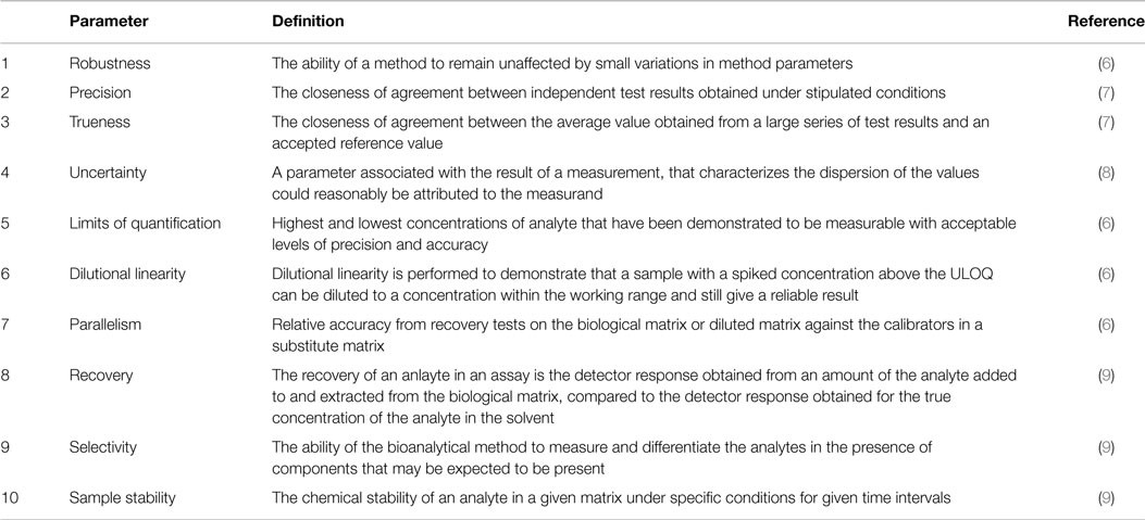Table 1. Short description of the validation parameters for which SOPs are presented.