Kinetic Monte Carlo (KMC) simulations have become a powerful tool for understanding and predicting the dynamics of various phenomena, especially in surface science. This comprehensive guide offers a practical guide to surface kinetic Monte Carlo simulations, focusing on lattice KMC methods widely used in surface and interface applications. It provides in-depth explanations, worked-out examples using the kmos code, and highlights critical approximations and potential pitfalls in implementing KMC models. The guide covers applications such as surface diffusion, crystal growth, and heterogeneous catalysis, addressing both transient and steady-state kinetics.
1. Introduction to Kinetic Monte Carlo Simulations
Monte Carlo methods utilize random numbers to solve complex problems. Kinetic Monte Carlo (KMC) extends this concept to simulate the dynamical properties of systems. In atomistic simulations, KMC acts as a coarse-graining technique, bridging the gap between microscopic elementary processes and meso- to macroscopic behaviors. KMC is invaluable in hierarchical multiscale modeling, where information from different levels of detail is integrated for a comprehensive description.
Consider heterogeneous catalysis as an example. Designing a catalytic process requires understanding phenomena from reactive chemistry to heat and mass transport. Numerical simulations, especially KMC, are integral to this design process, requiring models at multiple time and length scales.
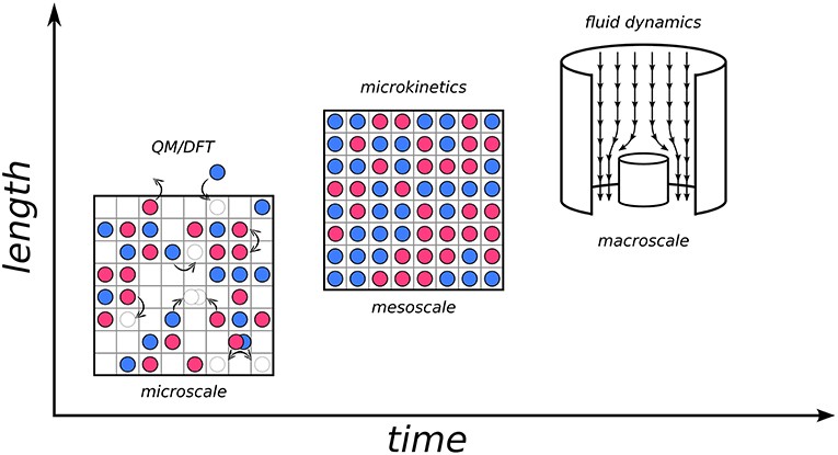
Figure 1 illustrates this multiscale approach.
Figure 1. Diagram illustrating the three scales in a hierarchical multiscale approach to heterogeneous catalysis. Microscale depicts elementary processes; mesoscale shows the interplay of these processes on surface composition and activity; macroscale illustrates fluid flow in a reactor.
Moving from the macroscale (industrial reactor) down to the microscale, events are governed by electronic structure: adsorption, desorption, diffusion, bond breaking, and bond forming. These elementary processes are described using the Potential Energy Surface (PES) of the system, often calculated using Density-Functional Theory (DFT).
“Zooming out” to the mesoscopic scale reveals the collective behavior resulting from the interplay of elementary processes and the surrounding environment. Here, microkinetic models, including KMC, are employed to capture the spatiotemporal evolution at the interface.
Finally, at the macroscale, transport phenomena and gradients are considered using continuum-type fluid dynamical models. Information from microkinetic models is integrated as input, e.g., as a boundary condition. Developing effective hierarchical models and “bridges” to transfer information is crucial for modern multiscale modeling.
Similar approaches are applied in diffusion and crystal growth, focusing on surfaces and interfaces. This guide concentrates on KMC techniques in these application areas, providing a practical approach with best practice recommendations, current challenges, and perspectives.
2. KMC Simulations: Theory to Codes
2.1. Rare-Event Dynamics
Many elementary processes on solid surfaces involve high activation barriers, classifying them as rare events. While atomic motions occur on picosecond timescales, the time between high-barrier events can be much longer. The system spends most of its time vibrating around a single minimum on the PES. Transitions to other (meta)stable states occur only occasionally. Thus, the time evolution manifests as a series of jumps from state to state. After spending considerable time in a basin, the system “forgets” how it got there, and each escape becomes independent of the preceding history, forming a Markov chain.
Figure 2 illustrates the coarse-graining of a molecular dynamics (MD) trajectory into a Markov chain.
Figure 2. The process of coarse-graining a molecular dynamics (MD) trajectory into a Markov chain, representing transitions between PES minima.
The change in probability *Pi(t) of the system being in state i at time t depends on the probabilities of hopping out of state i into any other state j, kij, and into state i from any other state j, kji. These hopping probabilities are expressed as rate constants. The overall change in Pi(t*) is governed by the Markovian master equation:
dPi(t)dt=-∑j≠ikijPi(t)+∑j≠ikjiPj(t). (1)
Solving Equation (1) explicitly becomes unfeasible due to the vast number of possible states. The Monte Carlo idea behind KMC avoids dealing with the entire matrix, instead generating stochastic trajectories that propagate the system from state to state. The correct time evolution of the probabilities *P*i(t) is obtained by averaging over these trajectories. The KMC method replaces the analytical solution of Equation (1) with a numerical approach based on stochastic dynamics. The algorithm determines the next state and the time step for the next jump.
2.2. Mapping onto a Lattice: Lattice KMC
Challenges in applying KMC practically relate to the numerous minima on PESs and the even larger number of connecting elementary processes. Ideally, rate constants calculated from first principles would be used, but this is often not feasible due to computational costs.
Lattice KMC implementations exploit crystalline order, mapping PES minima onto a periodic lattice. System states differ only in their distribution of adsorbates on lattice positions. For example, consider the diffusion of an adatom on an fcc(100) surface. If stable PES minima correspond to fourfold hollow sites, a lattice model can be established including only diffusion processes that allow the adatom to start and end up in one of the lattice sites.
Translational symmetry of a crystalline lattice can further reduce the number of required rate constants. In the diffusion example, the elementary processes out of any hollow site are the same. Computing the rate constants once allows reusing them for other hollow sites. Near-sightedness of chemical interactions also helps: the interaction with nearby species may have a negligible influence on the rate constant.
Lateral interactions of adsorbates with species in nearest-neighbor sites can be considered. As illustrated in Figure 3, in the diffusion example, five distinct rate constants are needed, one for each possible occupation of the four nearest neighboring sites.
Figure 3. Illustration of the hopping diffusion process on a quadratic lattice considering nearest neighbor configurations.
The lattice approximation allows scanning all possible configurations and transitions, computing associated rate constants beforehand and saving them in a rate catalog.
The approximations used can be efficient and allow for large supercells. However, detailed PES information is required, and an ordered lattice is assumed. Any changes of the lattice induced by simulated processes cannot be captured. Off-lattice KMC overcomes such limitations.
2.3. Mean-Field Approximation
An alternative to the full numerical solution of the Master equation with KMC is the mean-field approximation (MFA). This sacrifices the detailed spatial resolution over the extended lattice, replaced by the mean coverage of each considered species at any of the site types. The MFA assumes that the occupation of different sites on the lattice is statistically independent, i.e., no correlations exist between different sites.
The (time-dependent) rate *r*ij(t) of an elementary process is given by:
rij(t)=Pi(t)kij. (2)
Considering only first- and second-order processes, the pair-probability of finding species A at site a and species B at a neighboring site b with *P*ab(A, B, t) is:
Pab(A,B,t)=Θa(A,t)Θb(B,t), (3)
where Θa(A, t) and Θb(B, t) are the spatially averaged coverages of species A at sites of type a and species B at sites of type b, respectively.
Generalizing this to any reaction order, the MFA condenses the high-dimensional Master equation into rate equations of the form:
rij(t)=Nijkij∏a∈iΘa(A,t), (4)
where *N*ij is a geometrical factor.
The MFA yields a set of coupled differential equations solvable by standard algorithms. This is often combined with assumptions about the rate-determining step to arrive even at an analytical solution for the reaction rate.
While the MFA simplifies the problem, it represents an approximation generally only fulfilled for infinitely fast diffusion and in the complete absence of lateral interactions.
2.4. KMC Codes
Several high-end KMC codes have appeared recently. Some prominent examples include:
- CARLOS: Allows specifying any kind of reaction and uses pattern recognition to identify possible reactions.
- SPPARKS: Implements several KMC solvers and is structured modularly.
- ZACROS: Incorporates cluster expansion Hamiltonians to accurately account for long-range lateral interactions.
- MonteCoffee: Uses neighbor lists to represent site connectivity, geared toward nanoparticle simulations.
- EON: Includes algorithms to model mesoscale dynamics and implements a server-client architecture for aKMC.
- kmos: An application programming interface-based KMC framework that facilitates the generation of abstract model definitions in Python, then used to automatically generate efficient Fortran code.
The KMC algorithm underlying kmos is further described in the following section as one example of present-day codes.
3. Getting Practical: KMC Algorithms and Input Data
The KMC algorithm generates stochastic trajectories to yield the time evolution of the probability *P*i(t) in the Master Equation (1). The BKL algorithm (or “n-fold way,” Variable Step Size Method, Direct Method) is commonly used.
For a system with only two states A and B connected by a barrier with rate constants *kAB and kBA, the probability distribution p*AB for the true time of first escape is:
pAB(t)=kABexp(-kABt). (5)
The system clock is advanced by:
ΔtAB=-ln(ρ2)kAB, (6)
where ρ2 ∈ [0, 1] is a randomly drawn number.
Generalizing to an arbitrary system with multiple possible processes i → j, the time until any process has occurred is:
Δtescape=-ln(ρ2)ktot, (10)
where ρ2 ∈ [0, 1] is a randomly drawn number and
ktot=∑jkij (9)
is the total escape rate constant.
The BKL algorithm determines the executed process by drawing a random number ρ1 and multiplying it by ktot. The resulting number “points” at the process with correct probability.
Figure 4 illustrates this algorithm and the random process selection.
(Left) Flowchart of the BKL algorithm as implemented in kmos. (Right) Graphical illustration of random process selection in the process stack.
The algorithm can be summarized as follows:
- Make a list of possible processes p for the system to escape the current state i, with associated rate constants *k*p;
- Draw two random numbers ρ1, ρ2 ∈ [0, 1];
- Calculate ktot=∑pkp;
- Extract process q, which has to fulfill the constraint ∑p=1qkp≥ρ1ktot≥∑p=1q-1kp;
- Execute randomly drawn process;
- Update clock: t → t − ln(ρ2)/ktot.
4. Rate Constants from First Principles: Transition State Theory
KMC requires rate constants for all considered elementary processes. For surface applications, these are predominantly obtained through Transition State Theory (TST). Assuming no-recrossing and purely classical barrier crossing, TST provides the Eyring equation:
kijTST=qTSvibqivibkBThexp(-ΔEijkBT)=kokBThexp(-ΔEijkBT), (11)
where T is the absolute temperature, h is Planck’s constant, qTSvib and qivib are the partition functions at the transition state and initial state, respectively, and Δ*E*ij is the activation barrier.
Harmonic TST is most popular, where partition functions are obtained from vibrational modes. However, the computational costs of these calculations are often avoided, and one approximates *k*o ≃ 1 − 10, yielding a prefactor in the range 1012 − 1013 s−1.
For non-activated adsorption processes, the rate constant is better estimated as:
kn,Bads(T,pn)=S~n,B(T)pnAuc2πmnkBT, (12)
where *p*n is the partial pressure of species n of mass m, and the local sticking coefficient S~n,B(T).
4.1. Master Equation and Detailed Balance
In steady state, the Master equation leads to the condition:
∑j≠i[kijPi*-kjiPj*]=0, (13)
where Pi* (Pj*) is the time-independent probability.
At thermodynamic equilibrium, the principle of detailed balance imposes:
kijkji=Pj*Pi*. (14)
This is proportional to the states’ Boltzmann weights and can be expressed in terms of the free energy difference:
kijkji=exp(-Fj(T)-Fi(T)kBT). (15)
Every microscopic process must have a defined reverse process, and the rate constant expressions must fulfill Equation (15). Computing the free energies of both states *Fi and Fj* with the same numerical approximations is crucial for thermodynamic consistency.
4.2. Obtaining Rate Constants: Transition State Search
Locating the lowest activation barriers involves finding the lowest first-order saddle points on the PES.
4.2.1. Interpolation Methods
The simplest form of interpolation-based TS search involves identifying a reaction coordinate and constraining it to specific values while optimizing remaining degrees of freedom. These are coordinate-driving methods. The success depends on choosing good reaction coordinates.
Significant improvement is achieved by simultaneously optimizing multiple points along the reaction path, such as with the Nudged Elastic Band (NEB) method. After initializing a chain of images **R**i, NEB minimizes a target function:
SEB(R1,…,RN)=∑i=1NE(Ri)+∑i=1N-112k(Ri+1-Ri)2. (16)
The total force acting on each image is then:
Fi,NEB=Fi∥s-F⊥i=k(|Ri+1-Ri|-|Ri-Ri-1|)τ^i-∇E(Ri)⊥, (17)
In the Climbing-Image NEB (CI-NEB) variant, the image with the highest energy is driven up toward the saddle point.
4.2.2. Local Methods
Local methods locate transition states by minimizing the gradient norm. The Newton-Raphson (NR) approach locates the TS directly, provided the search starts sufficiently close to the TS.
The dimer method determines the direction along which the energy should be maximized without calculating the Hessian explicitly, employing two symmetrically displaced replicas–the dimer.
Figure 5 illustrates transition states and the NEB and dimer TS search methods.
(Left) An arbitrary PES exhibiting multiple minima. (Center) Illustration of the NEB method. (Right) Illustration of the dimer method.
4.2.3. BEP and Scaling Relations
The Brønsted-Evans-Polanyi (BEP) relation yields linear relationships of the kind:
ΔE≃c1(EFS-EIS)+c2, (18)
where c1 and c2 are constants and EFS and EIS are the total energies of the final and initial states.
Binding energies of reactants, products, and intermediates correlate with the binding energies of a few base elements. Such scaling relations, combined with BEP relations, enable an enormous reduction of the computational cost.
5. Garbage In – Garbage Out
Predictions are limited by the quality of input data. A KMC simulation depends on a fixed list of processes with rate constants that come with the typical uncertainty imposed by the underlying DFT calculation.
Advanced KMC approaches automatically identify relevant processes, but are generally more computationally demanding.
5.1. Adatom Diffusion on Au(100)
The simplest diffusion process consists of Au atoms hopping between 4-fold hollow adsorption sites on Au(100). A simple KMC model considers a (20 × 20) square lattice of adsorption sites. Possible processes are hops of particles from one site into one of the four neighboring sites. Neglecting lateral interactions, the barrier is ΔEdiff = 0.83 eV. The diffusion coefficient D can then be calculated as
D=〈MSD(t)-MSD0〉2dt, (19)
where t is the simulation time and d is the lattice dimension (2 in this case).
However, an alternative exchange diffusion mechanism exists, where a metal adatom replaces a surface layer atom and pushes it to a neighboring adsorption site. This occurs with a lower barrier of 0.65 eV on Au(100).
Figure 6 illustrates the hopping and exchange diffusion mechanisms.
(A) Illustration of the hopping diffusion mechanism. (B) Illustration of the exchange diffusion mechanism.
Including exchange diffusion dramatically changes the simulation output, as the barrier enters the rate constant exponentially.
Figure 7 plots the mean squared displacements and diffusion constants for both mechanisms.
Figure 7. Averaged mean squared displacements and diffusion constants of adatoms on Au(100) for hopping and exchange diffusion processes and various associated barriers.
This highlights the extent to which the outcome of a KMC simulation depends on knowing and allowing for all relevant processes.
6. Steady-State and Transient Simulations for Surface Catalysis
For catalysis, the behavior of the system once it reaches steady state is often of interest. Quantities of interest include the surface composition, reaction mechanisms, and production rates. Alternatively, the transient behavior of a system prepared in a given initial state might be of interest.
6.1. CO Oxidation on RuO2(110)
The CO oxidation model is taken from Reuter et al. (2004). The RuO2(110) surface contains two types of active sites, br (bridge) and cus (coordinately unsaturated) sites, arranged in an alternating rectangular lattice. A total of 26 processes are possible in this system, covering non-dissociative CO adsorption/desorption, dissociative O2 adsorption/desorption, diffusion of O and CO, as well as CO2 formation.
Figure 8 shows the structure of the RuO2(110) surface.
Figure 8. Top view of the structure of the RuO2(110) surface.
Figure 9A shows the temporal evolution of the system beginning from an empty lattice at 1 bar O2 and CO pressure and a temperature of 450 K. The system initially builds up coverage rapidly, but does not represent the true steady state. A prolonged simulation shows coverages changing dramatically, accompanied by a decrease in the TOF.
Figure 9B shows that starting from a completely different initial population (1 ML oxygen coverage on cus sites and vacant bridge sites) does lead to the same steady state, demonstrating the importance of exploring multiple initial conditions.
Figure 9. Temporal evolution of CO oxidation TOF and surface coverage on RuO2(110).
Once the steady-state solution has been reached, ergodicity can be used to calculate the desired quantities as time averages instead of ensemble averages.
7. Sensitivity Analysis and Uncertainty Quantification
It can be of particular interest to know the extent to which the rate constants of the various processes influence the model predictions and to thereby quantify the uncertainty of those predictions.
One sensitivity measure is Campbell’s degree of rate control (DRC) XRC, I for reaction step I:
XRC,I=kI〈rβ〉(∂〈rβ〉∂kI)kJ≠I,KI, (21)
where the average reaction rate 〈rβ〉 should be calculated for the product β of interest and the derivative is evaluated holding constant the rate constants *kJ of all other reactions steps J and the equilibrium constant KI for step I*.
Recent methods have been developed for global sensitivity analysis and UQ, to assess which conclusions about the model can be reliably drawn despite uncertainties in the input parameters.
8. Timescale Disparity Problem
KMC can face challenges when processes occur at largely different timescales. Most of the CPU time is spent simulating the fast processes, while the (maybe truly important) dynamics arising from the slow processes is sampled insufficiently or not at all.
Recent KMC works have often relied on simple acceleration schemes that function by decreasing the rate constants of the fastest processes. Algorithms have appeared that automatically scale fast processes.
The accelerated superbasin KMC (AS-KMC) method defines a superbasin as a set of lattice configurations that the system can jump between through the execution of quasi-equilibrated processes only.
Figure 10 illustrates the concept of superbasins and the approach of scaling rate constants.
Figure 10. Potential energy surface (PES) for a system with processes occurring at disparate timescales. The KMC simulation is accelerated by scaling the rate constants of fast, quasi-equilibrated processes.
9. Lateral Interactions
Lateral interactions are interactions between species adsorbed to a lattice.
Lateral interactions can be accounted for in lattice KMC models through the general cluster expansion method. The lattice energy is expanded into a sum of discrete interactions (clusters) through a lattice-gas Hamiltonian.
In practice, lateral interactions can be accounted for in lattice KMC models through the general cluster expansion method. In this method, the lattice energy is expanded into a sum of discrete interactions (clusters) such as pairwise interactions, three-body interactions etc. through a lattice-gas Hamiltonian. For any adsorbate on the lattice, one would thus evaluate how many neighbors of which type sit at which kind of distances (nearest-neighbor, next nearest neighbor etc.).
9.1. kmos Models with Lateral Interactions
The local smart backend offers the best runtime possible at the expense of memory usage, featuring a pre-calculated list of rate constants. The on-the-fly backend calculates rate constants on-the-fly instead of making use of a pre-calculated rate catalog.
As an example, consider a crystal growth model with attractive pairwise lateral interactions. The rate constant for the desorption process kdes becomes
kdes=kBThexp(-ΔE0+nNN·ϵintkBT), (22)
where nNN is the number of nearest neighbor species in the lattice configuration.
Figure 11A illustrates this lateral interaction model. Figure 11B shows snapshots of grown crystal structures at two different temperatures.
(A) Illustration of the lateral interaction model for the desorption process of the crystal growth model. (B) Snapshots of grown crystal structures at two different temperatures.
Returning to the CO oxidation model, Figure 11C illustrates possible pairwise interactions. Figure 11D shows kmos performance for the CO oxidation model as a function of the number of pairwise interactions considered for two different backends.
(C) Illustration of pairwise interactions in the CO oxidation on RuO2(110) model. (D) kmos performance for the CO oxidation model as a function of the number of pairwise interactions considered for two different backends.
10. Summary and Outlook
This guide has provided practical guidelines and examples for constructing and evaluating KMC models, highlighting pitfalls, challenges, and perspectives. We have covered the lattice approximation, off-lattice KMC, transition state theory, BEP and scaling relations, sensitivity analysis, the timescale disparity problem, and lateral interactions.
Future developments include cheaper methods for determining rate constants, improved sensitivity analysis, and better algorithms for addressing the timescale disparity problem. By addressing these challenges and continuing to refine KMC methodologies, we can achieve an improved understanding of surface phenomena and design novel materials and catalysts.